

printf("ho_tari\n");
PCA #8 본문
<코드>
from tensorflow.keras.datasets import cifar10
from tensorflow.keras.utils import to_categorical
from tensorflow.keras import models, layers
from tensorflow.keras.callbacks import EarlyStopping
import numpy as np
import matplotlib.pyplot as plt
# data loading
(X_train, Y_train), (X_test, Y_test) = cifar10.load_data()
# data preprocessing
X_train = X_train / 255.0
X_test = X_test / 255.0
num_classes=10
Y_train_ = to_categorical(Y_train, num_classes)
Y_test_ = to_categorical(Y_test, num_classes)
# model definition
L,W,H,C = X_train.shape
input_shape = [W, H, C] # as a shape of image
def build_model():
model = models.Sequential()
# first convolutional layer
model.add(layers.Conv2D(32, kernel_size=(3,3), activation='relu',
input_shape=input_shape))
# second convolutional layer
model.add(layers.Conv2D(64, (3,3), activation='relu'))
# max-pooling layer
model.add(layers.MaxPooling2D(pool_size=(2,2)))
model.add(layers.Dropout(0.25))
# Fully connected MLP
model.add(layers.Flatten())
model.add(layers.Dense(128, activation='relu'))
model.add(layers.Dropout(0.5))
model.add(layers.Dense(num_classes, activation='softmax'))
# compile
model.compile(optimizer='rmsprop', loss='categorical_crossentropy', metrics=['accuracy'])
return model
# main loop without cross-validation
import time
starttime=time.time();
num_epochs = 50
model = build_model()
history = model.fit(X_train, Y_train_, validation_split=0.2,
epochs=num_epochs, batch_size=100, verbose=1)
train_loss, train_acc = model.evaluate(X_train, Y_train_)
test_loss, test_acc = model.evaluate(X_test, Y_test_)
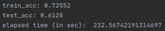
print('train_acc:', train_acc)
print('test_acc:', test_acc)
print("elapsed time (in sec): ", time.time()-starttime)
# visualization
def plot_acc(h, title="accuracy"):
plt.plot(h.history['acc'])
plt.plot(h.history ['val_acc'])
plt.title(title)
plt.ylabel('Accuracy')
plt.xlabel('Epoch')
plt.legend(['Training', 'Validation'], loc=0)
def plot_loss(h, title="loss"):
plt.plot(h.history ['loss'])
plt.plot(h.history ['val_loss'])
plt.title(title)
plt.ylabel('Loss')
plt.xlabel('Epoch')
plt.legend(['Training', 'Validation'], loc=0)
plot_loss(history)
plt.savefig('chapter5-1_cifar10.loss.png')
plt.clf()
plot_acc(history)
plt.savefig('chapter5-1_cifar10.accuracy.png')
Q1
Start with chapter5_1_cifar10.py and modify the code as follows.
We will add “Dropout” layers after the max-pooling layer and the hidden layer of MLP. Add the following lines to the right locations.
model.add(layers.Dropout(0.25)) # after max-pooling
model.add(layers.Dropout(0.5)) # after the hidden layer of MLP
Show the modified “build_model” function.
<코드>

Q2
When we use the dropout, we need more time to learn the model. So, please increase the number of maximum epochs to 50.
Run the code. Attach the loss graph. And What was the test accuracy?
Loss graph
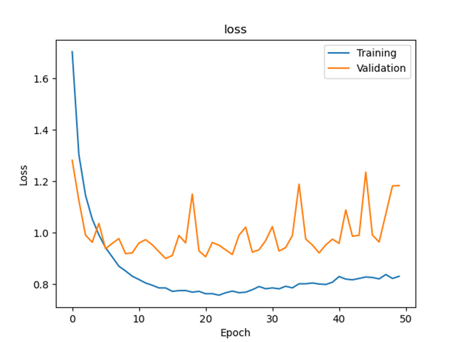
Final test accuracy:

Q3
The learning curve of Q2 may be oscillating.
Maybe it’s better to decrease the learning rate. Change the learning rate of RMSprop to 0.0001. Also, the smaller size of minibatch also helps to stabilize the learning procedure. Set minibatch to 32. (it will increase the learning time about three times)
Run the code. Attach the loss graph. What was the test accuracy?
Loss graph

Final test accuracy:


Q4
The other approach of machine learning is “high-capacity model with strong regularization”.
Indeed, it is not recommended to add dropout layers to the small-sized NN model. Do you think our current model is large enough? Is there any chance that our model is underfitting? Maybe not. However we did not check it.
Let’s test it.
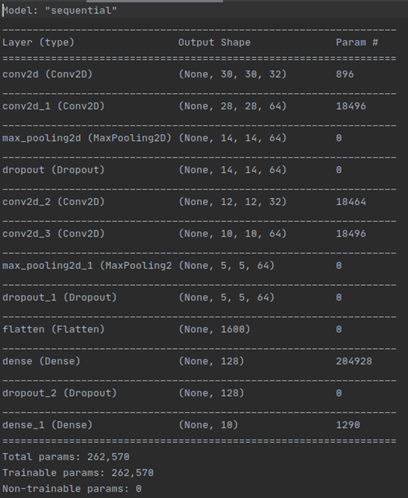
To test it, let’s increase model capacity (See the guideline for details). Since the model becomes more complex, we need more time to learn. Set the number of maximum epochs to 100.
Run the code. Attach the loss graph. What was the test accuracy?
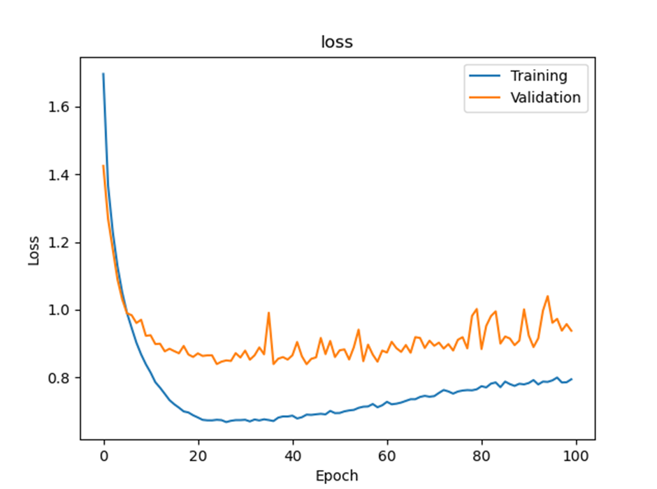
Loss graph
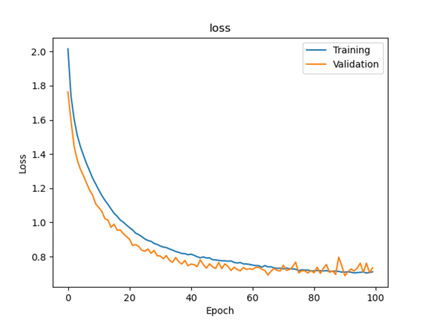
Final test accuracy:

Q5
There is another possible way to have “high-capacity model”.
Let’s try to increase the number of hidden neurons in MLP four times (512) without adding convolution layers (See guideline.)
Run the code. Attach the loss graph. What was the test accuracy?
Loss graph
Final test accuracy:

Q6
You have 4 sets of loss graphs and test accuracy with different learning scheme.
Which one was the best? And why do you think so? (Consider various factors including the number of parameters, total learning time, and final performance.)
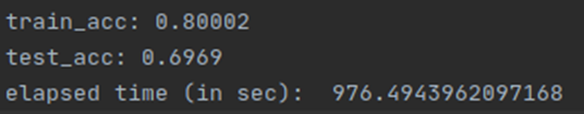
Q4에서 한 conv2d layers, max pooling layers and dropout layers를 한 번씩 더 진행시킨 “High-capacity model with strong regularization”방법이 제일 좋다고 생각합니다. Total parameters 수를 비교해보면 Q2,3에서는 1,626,442개이고 Q4에서는 262,570개이며 Q5에서는 6,447,562개로 나와 Q4에서 제일 적고 Q5에서 제일 많은 것을 알 수 있습니다. Total learning time을 비교해보면 Q2에서는 대략 233초정도, Q3에서는 대략 414초정도, Q4에서는 대략 989초, Q5에서는 대략 976초정도로 나와 Q4에서 제일 오래 걸리고 Q2에서 제일 빠른 것을 알 수 있습니다. Final performance로 test accuracy를 비교해보면 Q2에서는 0.6128, Q3에서는 0.6913, Q4에서는 0.7581 그리고 Q5에서는 0.6969정도가 나와 Q4에서 제일 높고 Q2에서 제일 낮은 것을 알 수 있었습니다. Loss graph를 비교해보면 Q2에서는 진동이 크게 일어나며 loss가 다른 방법에 비해 높게 나오는 것을 알 수 있으며 Q3에서는 loss값이 작게 나오긴 하지만 진동이 살짝 크게 있는 편으로 나왔습니다. Q4에서는 Q3과 마찬가지로 loss값이 비교적 낮게 나왔으며 진동이 있긴 하지만 진동폭이 비교적 작게 나온 것을 알 수 있고 Q5에서는 loss값이 크게 나오고 점점 위로 올라가는 모습으로 보아 overfitting이 일어나는 것으로 보입니다. 따라서 accuracy가 제일 높고 loss값이 작으며 그나마 steady하게 나오는 Q4 방법이 가장 좋은 것 같습니다.
Extra Question
You will see two different training accuracy.
One is the training accuracy of the last epoch during the learning phase, which is drawn in the accuracy graph and is generally around 0.75.
The other is the value after “train_acc: XXX”, which is the results of “model.evaluate()” and is slightly larger than the former one (~0.80).
Why are they different?
첫 번째는 train data를 model이 직접 학습하면서 weight와 bias를 업데이트하면서 성능을 높이는 경우이다. 학습시키는 과정에서 에러가 최소인 지점을 찾기 위해서 계속 parameter의 값들이 업데이트된다. 이때 local minima에 stuck되는 현상 등을 피하기 위해서 weight의 변화를 주면서 학습된다. 따라서 epoch마다 마지막 training accuracy는 다양하게 나온다.
두 번째는 이미 학습을 마친 model을 통해서 evaluation하여 얻은 결과이다. 따라서 이미 학습된 성능이 발전한 model에 train data를 넣어 시험을 통해 training accuracy를 출력한다. 따라서 model.evaluate(train data)을 사용하여 얻은 training accuracy는 학습하는 과정에서 얻은 마지막 training accuracy보다 조금 더 증가하였다.


