PCA #9

<코드>

from tensorflow.keras.preprocessing.image import ImageDataGenerator
from tensorflow.keras import models, layers, optimizers
from tensorflow.keras.callbacks import EarlyStopping
import matplotlib.pyplot as plt

# set image generators
train_dir='./datasets/cats_and_dogs_small/train/'
test_dir='./datasets/cats_and_dogs_small/test/'
validation_dir='./datasets/cats_and_dogs_small/validation/'

train_datagen = ImageDataGenerator(rescale=1./255)
validation_datagen = ImageDataGenerator(rescale=1./255)
test_datagen = ImageDataGenerator(rescale=1./255)

train_generator = train_datagen.flow_from_directory(
        train_dir,
        target_size=(150, 150),
        batch_size=20,
        class_mode='binary')
test_generator = test_datagen.flow_from_directory(
        test_dir,
        target_size=(150, 150),
        batch_size=20,
        class_mode='binary')
validation_generator = validation_datagen.flow_from_directory(
        validation_dir,
        target_size=(150, 150),
        batch_size=20,
        class_mode='binary')

# model definition
input_shape = [150, 150, 3] # as a shape of image
def build_model():
    model=models.Sequential()
    model.add(layers.Conv2D(32, (3, 3), activation='relu',
                            input_shape=input_shape))
    model.add(layers.MaxPooling2D((2, 2)))
    model.add(layers.Conv2D(64, (3, 3), activation='relu'))
    model.add(layers.MaxPooling2D((2, 2)))
    model.add(layers.Conv2D(128, (3, 3), activation='relu'))
    model.add(layers.MaxPooling2D((2, 2)))
    model.add(layers.Conv2D(128, (3, 3), activation='relu'))
    model.add(layers.MaxPooling2D((2, 2)))
    model.add(layers.Flatten())
    model.add(layers.Dense(512, activation='relu'))
    model.add(layers.Dense(1, activation='sigmoid'))
    # compile
    model.compile(optimizer=optimizers.RMSprop(lr=1e-4),
                  loss='binary_crossentropy', metrics=['accuracy'])
    return model

# main loop without cross-validation
import time
starttime=time.time();
num_epochs = 60
model = build_model()
history = model.fit_generator(train_generator,
                    epochs=num_epochs, steps_per_epoch=100,
                    validation_data=validation_generator, validation_steps=50)

# saving the model
model.save('cats_and_dogs_small_1.h5')

# evaluation
train_loss, train_acc = model.evaluate_generator(train_generator)
test_loss, test_acc = model.evaluate_generator(test_generator)
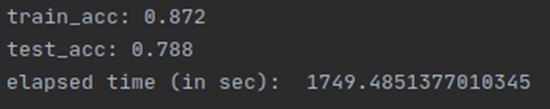
print('train_acc:', train_acc)
print('test_acc:', test_acc)
print("elapsed time (in sec): ", time.time()-starttime)

# visualization
def plot_acc(h, title="accuracy"):
    plt.plot(h.history['acc'])
    plt.plot(h.history ['val_acc'])
    plt.title(title)
    plt.ylabel('Accuracy')
    plt.xlabel('Epoch')
    plt.legend(['Training', 'Validation'], loc=0)

def plot_loss(h, title="loss"):
    plt.plot(h.history ['loss'])
    plt.plot(h.history ['val_loss'])
    plt.title(title)
    plt.ylabel('Loss')
    plt.xlabel('Epoch')
    plt.legend(['Training', 'Validation'], loc=0)

plot_loss(history)
plt.savefig('chapter5-2_basic.loss.png')
plt.clf()
plot_acc(history)
plt.savefig('chapter5-2_basic.accuracy.png')

 

Q1 

(Start with Chatper5_2.py and modify it.)

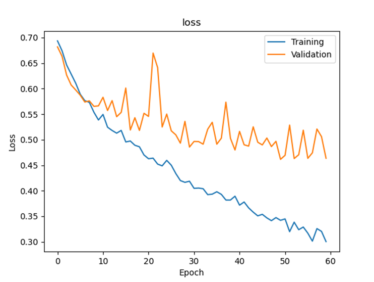
Increase the number of epochs to “60”.

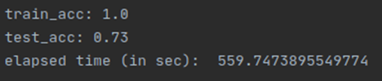
Run the code. Attach its loss graph. What is the test accuracy?

It requires data preparation. In other words, this question is scoring your data preparation.

 

Loss graph

Final test accuracy:

 

Q2 

(Keep working with Chatper5_2.py. We will modify it.)

Using the code in the slide 19 of CNN(5), add “data augmentation” to the train_datagen.

Set the number of epochs to “60”.

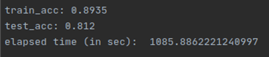
Run the code, and attach its loss graph. What was the test accuracy?

 

Loss graph

Final test accuracy:

 

Q3 

(Keep modifying Chatper5_2.py)

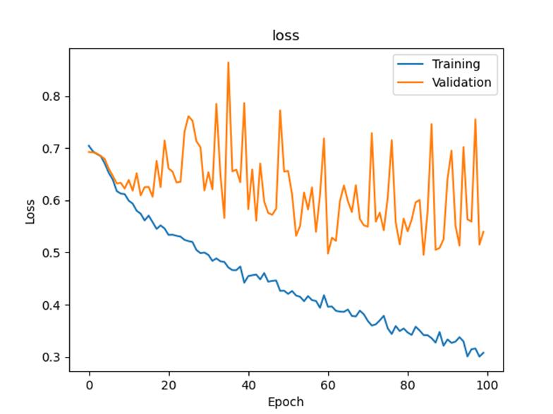
Let’s add dropout layers after every maxpool layers with 0.25 dropout probability. (We have 4 maxpool layers; thus, you will have 4 dropout layers). Set the number of epochs to “100”.

Run the code. Attach its loss graph. What was the test accuracy?

 

Loss graph

Final test accuracy:

 

Q4 

Which one was the best among the results of Q1-Q3 in terms of overfitting? What do you conclude from the results (Q1-Q3)

 

Test accuracy를 비교해 보았을 때 Q2 > Q3 > Q1으로 나타나 Q2가 가장 좋다고 생각합니다. Q1의 loss 그래프를 보면 오른쪽 위로 상향하는 것으로 overfitting이 일어나고 있다는 것을 알 수 있습니다. Q2의 상황에서는 Q1의 상황에서 data augmentation을 추가하였고 training accuracy는 Q1에 비해 줄어들었지만 test accuracy는 더 커진 결과를 알 수 있습니다. 또한, epoch에 대한 loss 그래프를 보아 overfitting을 예방했다고 볼 수 있는 것 같습니다. Q3의 상황에서는 data augmentation과 dropout을 같이 사용하여 결과를 확인하는 것인데 epoch을 100으로 늘려 진행하여 Q1에 비해 train accuracy는 낮아지고 test accuracy는 높아지는 결과를 볼 수 있지만 학습 시간이 늘어나면서 overfitting을 완전히 예방하지 못한 것으로 보입니다. 따라서 overfitting을 예방하고 가장 높은 test accuracy를 보인 Q2가 가장 좋다고 생각합니다.