HW2

Breast Cancer Wisconsin Dataset

 

Classification problem

◦ 10 input variables

◦ 1 binary output variable (benign or malignant)

 569 data samples

◦ Use the first 100 samples as test set

◦ Use the next 100 samples as validation set

◦ Use the others as training set

◦ Use Numpy slicing. Do not use the “train_test_split” function.

 

Data Preparation

 

Download breast-cancer-wisconsin.data

 Remove the rows with missing values “?”

◦ With any text editor

 Load it in the python

 Drop the first column:

◦ The first column is ID, which does not carry any information about the tissue.

 Normalize the input variables.

 Set the output variable ◦ Set Malignant: 1, benign: 0

 Data split: train, test, & validation set

◦ Use Numpy slicing. Do not use the “train_test_split” function.

 

Basic Model

 

Model Structure

◦ 9 inputs

◦ 10 hidden neurons with ReLu activation functions

◦ 1 output neuron with sigmoid activation function.

 Compile and learning condition

◦ Optimizer=rmsprop,

◦ Loss function=binary crossentropy

◦ Epochs=200

◦ Batch_size=10

◦ EarlyStopping with patience=2

 

Q1

<코드>

import pandas as pd
import numpy as np
from sklearn.preprocessing import MinMaxScaler
from tensorflow.keras.models import Sequential
from tensorflow.keras.layers import Dense
from tensorflow.keras.callbacks import EarlyStopping

# 데이터파일 load
cancer = pd.read_csv("C:/Users/chank/PycharmProjects/pythonProject10/breast-cancer-wisconsin (1).data", delimiter=",")

# remove the rows with missing values "?"
for label in cancer:
    for index, data in enumerate(cancer.loc[:, label]):
        if data == "?":
            cancer = cancer.drop(index)

# output variable 설정
cancer.index = range(0, len(cancer))

for index, data in enumerate(cancer['2.1']):
    if data == 2:
        cancer['2.1'][index] = 0
    elif data == 4:
        cancer['2.1'][index] = 1

# 입력 변수와 출력 변수를 나눔
X = cancer.iloc[:, :-2].values
y = cancer.iloc[:, -1].values

# drop the first column
scaler = MinMaxScaler()
norm_cancer = scaler.fit_transform(X)
cancer = np.delete(norm_cancer, 0, axis=1)

# 테스트 세트, 검증 세트, 훈련 세트로 나눔
X_test = X[:100]
y_test = y[:100]
X_val = X[100:200]
y_val = y[100:200]
X_train = X[200:]
y_train = y[200:]

# 입력 변수를 표준화
X_train = scaler.fit_transform(X_train)
X_val = scaler.transform(X_val)
X_test = scaler.transform(X_test)

# Define the model
model = Sequential()
model.add(Dense(10, activation='relu', input_shape=(9,)))
model.add(Dense(1, activation='sigmoid'))

# Compile the model
model.compile(optimizer='RMSprop', loss='binary_crossentropy', metrics=['binary_accuracy'])

# Set early stopping callback
early_stopping = EarlyStopping(monitor='val_loss', patience=2)

# Train the model
history = model.fit(X_train, y_train, epochs=200, batch_size=10, validation_data=(X_val, y_val), callbacks=[early_stopping])

# 훈련 데이터에 대한 손실 및 정확도 계산
train_loss, train_accuracy = model.evaluate(X_train, y_train)

# 테스트 데이터에 대한 손실 및 정확도 계산
test_loss, test_accuracy = model.evaluate(X_test, y_test)

print("Training Loss:", train_loss)
print("Training Accuracy:", train_accuracy)
print("Test Loss:", test_loss)
print("Test Accuracy:", test_accuracy)

 

Q2

Repeat training of the model 5 times, and collect their losses and accuracies using the table

	Trial #1	Trial #2	Trial #3	Trial #4	Trial #5
Training Loss	0.07731712609529495	0.07346681505441666	0.07664284110069275	0.07194381952285767	0.07287615537643433
Training Accuracy	0.9730290174484253	0.9751037359237671	0.9751037359237671	0.9751037359237671	0.9751037359237671
Test Loss	0.2534460425376892	0.22062622010707855	0.23076114058494568	0.24551278352737427	0.21993254125118256
Test Accuracy	0.8700000047683716	0.8799999952316284	0.8600000143051147	0.8700000047683716	0.8700000047683716

Training Loss 값을 비교해보면 0.07대를 왔다갔다하는 모습을 볼 수 있어 비교적 일관성이 있게 나오는 것 같습니다.

Training Accuracy 값을 비교해보면 5번의 값이 모두 동일하여 일관성 있게 나오는 것을 알 수 있습니다.

Test Loss 값을 비교해보면 0.2대를 왔다갔다하는 모습을 보이며 비교적 일관성 있게 나오는 것 같습니다.

Test Accuracy 값을 비교해보면 0.87대의 값으로 비슷하게 나오는 것으로 보아 비교적 일관성이 있다고 생각합니다.

 

Q3

Investigate whether the activation function of the hidden layer affects the accuracy.

◦ Still the same model (the # of hidden neurons: 10)

◦ 4 different cases: None, Relu, sigmoid, tanh

◦ For each case, repeat training 10 times and report the mean and standard deviation of loss and accuracy in the training and test data set.

◦ Use the similar table in the problem #2.

◦ Collecting data

 Which one is the best? Why?

 

	None	Relu	Sigmoid	tanh
Training Loss	0.07189620374178886 ± 0.0022673122157215065	0.07176601415848732 ± 0.003039182205974641	0.07061661685752869 ± 0.0019501671287832236	0.07384743048477173 ± 0.0032562020640764654
Training Accuracy	0.9757775467634201 ± 0.0008684522385652002	0.9757943818569184 ± 0.0008704521773197296	0.9753215546607971 ± 0.001081264825594693	0.9757326002120972 ± 0.0008751202097064292
Test Loss	0.2293862602710724 ± 0.02110318188993305	0.2221267751455307 ± 0.011406303478186167	0.17000890612602235± 0.005221497599285532	0.20184976816153526 ± 0.023098091985450826
Test Accuracy	0.8679999943971634 ± 0.0066670758620308	0.8769999980926513 ± 0.008539059722967232	0.9180000185966492 ± 0.00871779776213976	0.8909999961853028 ± 0.018564800390408766

Training Loss를 비교해보았을 때 Sigmoid 활성화 함수를 썼을 때가 0.0706정도로 가장 낮게 나왔습니다.

Training Accuracy를 비교해보았을 때는 4가지 활성화 함수들이 모두 일관성 있게 나왔습니다.

Test Loss를 비교해보았을 때 Sigmoid 활성화 함수를 사용했을 때 0.17 정도로 가장 낮게 나왔습니다.

Test Accuracy를 비교해보았을 때 Sigmoid 활성화 함수를 사용했을 때 0.918 정도로 가장 높게 나온 것을 확인할 수 있었습니다.

위 값들의 비교 결과 Sigmoid 활성화 함수를 사용했을 때 Loss가 가장 낮고 Accuracy가 가장 높은 것을 알 수 있어 Sigmoid가 가장 좋다고 생각합니다.

 

Q4

Let’s investigate how the number of hidden neurons affects the performance.

◦ Set the activation function of the hidden layer to Relu.

 Change # of hidden neurons systematically, and then re-training the model.

◦ Collect the data and construct the table for the following # of hidden neurons: 2, 5, 10, 20, 50, 100, 200, 500, 1000, 2000.

◦ For each case, repeat training 5 times and report the mean and standard deviation of loss and accuracy in the training and test data set.

◦ 1 points for collecting data.

 What is the best case? Why did you select it? (i.e. which one did you use among 4 metrics you collected?)

	2	5	10	20	50
Training Loss	0.07723694054850174 ± 0.0017177856485469795	0.07263822212540063 ± 0.002472705659287289	0.07386304500700256 ± 0.002107431905655217	0.0682999656093846 ± 0.003379143158319959	0.07121228025116041 ± 0.002425229657691354
Training Accuracy	0.9751037359237671 ± 0.00080	0.9753322677612305 ± 0.0009228579020363495	0.9751037359237671 ± 0.0011079766651273154	0.9769484796466827 ± 0.0005600118898412227	0.9769489998817444 ± 0.0009814167076453828
Test Loss	0.2320204800033631 ± 0.007231978422354856	0.2189318648977561 ± 0.01918326230171072	0.2246534698009491 ± 0.018129104933280794	0.21548356767961104 ± 0.008030754858625416	0.22930492728900908 ± 0.013758235717871386
Test Accuracy	0.8799999952316284 ± 0.011547005383792416	0.8760000104904175 ± 0.014387846149345084	0.8759999871253968 ± 0.01154700542329235	0.8899999809265137 ± 0.010954451477388045	0.8740000123977661 ± 0.010954451150648883

 

	100	200	500	1000	2000
Training Loss	0.06937130680769405 ± 0.002402406234670626	0.06862617611980438 ± 0.0026340157800120147	0.0687240719795227 ± 0.004073763381798035	0.06758404895051834 ± 0.0023181592207318065	0.07016092524165885 ± 0.007202402483872522
Training Accuracy	0.9767430200576782 ± 0.0009178408892192456	0.9763886113166809 ± 0.000855259765408738	0.9757380557060242 ± 0.0008309427594804367	0.9769634103775024 ± 0.0006548657310781505	0.9757186431884766 ± 0.0016093252889458933
Test Loss	0.22407415987491607 ± 0.01219434532700335	0.23410523772239685 ± 0.018283322674002964	0.24395044565296173 ± 0.04549280435689885	0.26234699726104737 ± 0.02445027497548025	0.2853602135181427 ± 0.05646862346605097
Test Accuracy	0.8820000057220458 ± 0.011704699747463877	0.8720000147819519 ± 0.01341640772004274	0.8759999873638153 ± 0.02179430105092576	0.8640000100135803 ± 0.012247448212310783	0.8549999952316284 ± 0.02081666324770243

 

Training Date보다 Test Date를 비교해보는 것이 좋을 것 같아 Test Loss와 Test Accuracy를 보면서 값들을 비교해 보았습니다.

Test Loss 값을 비교해보면 hidden neuron의 개수가 20일 때가 0.215정도로 가장 낮은 것을 알 수 있습니다. 그 다음으로는 hidden neuron의 개수가 5일 때가 0.218정도로 낮게 나왔습니다.

Test Accuracy 값을 비교해보면 hidden neuron의 개수가 20일 때가 0.889정도로 가장 높게 나왔습니다. 두 번째로는 hidden neuron의 개수가 100일 때다 0.882정도로 높게 나왔습니다.

Test Loss가 가장 낮고 Test Accuracy가 가장 높은 hidden neuron의 개수가 20일 때가 가장 결과가 좋다고 생각합니다.

또한 회귀 문제는 일반적으로 모델이 예측한 값과 실제 값 간의 오차를 최소화하는 것이 목적이기 때문에 Test Loss를 기준으로 비교하는 것이 가장 좋다고 생각합니다.

따라서 Test Loss가 가장 낮은 hidden neuron이 20일 때가 가장 결과가 좋다고 생각합니다.

 

QE1

Generally, after performing the rough search we did in the Q4, we performed the more fine-tuned search for the optimal # of hidden neurons.

◦ As an example, if we found that the best performance was achieved near 20~50, we performed another experiment varying # of hidden neurons: 25, 30, 35, 40, 45, and select the case with the best performance.

 The question is “why didn’t we try all cases at once?”

◦ As an example, we can try for all cases: 2, 5, 10, 15, 20, 25, 30, 35, 40, 45, 50, 55, 60 ….

◦ But we don’t. Why?

 

<코드>

import pandas as pd
import numpy as np
from sklearn.preprocessing import MinMaxScaler
from tensorflow.keras.models import Sequential
from tensorflow.keras.layers import Dense
from tensorflow.keras.callbacks import EarlyStopping

# 데이터파일 load
cancer = pd.read_csv("C:/Users/chank/PycharmProjects/pythonProject10/breast-cancer-wisconsin (1).data",
                         delimiter=",")
# remove the rows with missing values "?"
for label in cancer:
    for index, data in enumerate(cancer.loc[:, label]):
        if data == "?":
                cancer = cancer.drop(index)

# output variable 설정
cancer.index = range(0, len(cancer))

for index, data in enumerate(cancer['2.1']):
    if data == 2:
        cancer['2.1'][index] = 0
    elif data == 4:
        cancer['2.1'][index] = 1

# 입력 변수와 출력 변수를 나눔
X = cancer.iloc[:, :-2].values
y = cancer.iloc[:, -1].values

# drop the first column
scaler = MinMaxScaler()
norm_cancer = scaler.fit_transform(X)
cancer = np.delete(norm_cancer, 0, axis=1)

print(cancer)

# 테스트 세트, 검증 세트, 훈련 세트로 나눔
X_test = X[:100]
y_test = y[:100]
X_val = X[100:200]
y_val = y[100:200]
X_train = X[200:]
y_train = y[200:]

# 입력 변수를 표준화
X_train = scaler.fit_transform(X_train)
X_val = scaler.transform(X_val)
X_test = scaler.transform(X_test)

# Define the model
model = Sequential()
model.add(Dense(1, activation='sigmoid', input_shape=(9,)))

# Compile the model
model.compile(optimizer='RMSprop', loss='binary_crossentropy', metrics=['binary_accuracy'])

# Set early stopping callback
early_stopping = EarlyStopping(monitor='val_loss', patience=2)

# Train the model
history = model.fit(X_train, y_train, epochs=200, batch_size=10, validation_data=(X_val, y_val),
                        callbacks=[early_stopping])

w = model.get_weights()[0]
b = model.get_weights()[1]

print(w)

print(b)

# 훈련 데이터에 대한 손실 및 정확도 계산
train_loss, train_accuracy = model.evaluate(X_train, y_train)

# 테스트 데이터에 대한 손실 및 정확도 계산
test_loss, test_accuracy = model.evaluate(X_test, y_test)

print("Training Loss:", train_loss)
print("Training Accuracy:", train_accuracy)
print("Test Loss:", test_loss)
print("Test Accuracy:", test_accuracy)

 

	25	30	35	40	45
Training Loss	0.07110340055844488 ± 0.0022201629074311837	0.07013595826244354 ± 0.002870501426505105	0.07225451819992065 ± 0.001966200121833307	0.06986976181251812 ± 0.004386212802358547	0.06911096727990127 ± 0.002039849108129921
Training Accuracy	0.9759444018424454 ± 0.0009040732733441467	0.9763332123756409 ± 0.0008259514547177072	0.9763332123756409 ± 0.0015496744750990842	0.976768271446228 ± 0.0009253294695972322	0.9769486529827117 ± 0.0008568379324342117
Test Loss	0.22296558144207917 ± 0.01567859657523912	0.21954829067993164 ± 0.014210236238325668	0.23047295770645143 ± 0.014420464726262957	0.22725796854162215 ± 0.014431333108896977	0.2247014313690424 ± 0.014215670414234238
Test Accuracy	0.8799999916553497 ± 0.014142136014378104	0.8740000128746033 ± 0.010954451455710528	0.28799999952316284 ± 0.00836660026534014	0.8859999897480011 ± 0.013038406723471938	0.8820000052452088 ± 0.01140175418965534

Hidden neuron의 개수의 비교 간격을 줄여서 학습을 시켜본 결과를 보면 개수를 10개 단위로 비교하는 것과 크게 다를 것이 없게 보입니다. 또한, 20에서 50사이로 개수를 지정하였을 때의 결과들이 서로 크게 다를 것이 없는 것으로 나타납니다. 따라서 굳이 2, 5, 10, 15, 20, 25, 30, 35, 40, 45, 50, 55, 60, …처럼 hidden neuron 개수 간격들을 좁게 하면 시간이 오래 걸릴 것으로 생각해서 개수 간격들을 2, 10, 50, 100, …정도로 해도 충분히 효율적으로 비교를 할 수 있을 것이라고 생각합니다.

 

QE2

After learning, we can analyze the learned weights.

 Construct a model without a hidden layer; all input units are directly corrected to the output.

 After learning, using the following commands, you can get the weights and bias.

◦ w=model.get_weights()[0]

◦ b=model.get_weights()[1]

 Please analyze the model based on the learned weights. What does the large weight mean? What does the weight near zero mean? What does the negative value mean?

 Check breast-cancer-wisconsin.names.

 

<히든 레이어를 없애고 모델링한 코드>

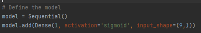
<weights와 bias 코드>          

<출력 결과>

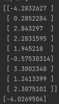
Weight의 값들과 입력 데이터를 분석해보면 다음과 같습니다.

Large weight란 입력과 출력 사이의 연결 강도가 크다는 것을 의미하는 “큰 가중치”입니다. 해당 입력이 출력에 큰 영향을 미친다는 것을 의미합니다. 모델에서 큰 가중치는 중요한 역할을 수행하는 입력과 출력 사이의 연결을 나타냅니다.

따라서 8. Bland Chromatin이 가장 큰 가중치를 가지고 있어 출력에 가장 큰 영향을 주는 것 같습니다. 그 외에 4. Uniformity of Cell Shape, 5. Marginal Adhesion, 6. Single Epithelial Cell Size, 9. Normal Nucleoli, 10. Mitoses 값들이 가중치가 1에서 3사이의 값이 나온 것으로 보아 그나마 큰 가중치에 속한다고 생각합니다.

Near zero mean weight란 해당 입력이 출력에 거의 영향을 미치지 않는 “0에 가까운 가중치”입니다. 모델에서 해당 입력과 출력 사이의 연결이 거의 없다는 것을 나타냅니다.

따라서 3. Uniformity of Cell Size는 weight가 이므로 0에 가까운 가중치를 가진 것 같습니다.

Negative value mean이란 해당 입력이 출력에 부정적인 영향을 미친다는 것을 의미하는 “음수 값 가중치”입니다. 해당 입력이 출력을 감소시키는 방향으로 영향을 미친다는 것을 나타냅니다.

따라서 2. Clump Thickness는 weight가 이고 7. Bare Nuclei는 weight가 이므로 음수 값 가중치를 가진 것 같습니다.