PCA #12

<코드>

from tensorflow.keras import layers, models
class AE(models.Model):
    def __init__(self, x_nodes=784, z_dim=36):
        x_shape = (x_nodes,)
        x = layers.Input(shape=x_shape)
        z = layers.Dense(z_dim, activation='relu')(x)
        y = layers.Dense(x_nodes, activation='sigmoid')(z)
    # Essential parts:
        super().__init__(x, y)
        self.compile(optimizer='adam', loss='binary_crossentropy', metrics=['accuracy'])
# Optional Parts: they are for Encoder and Decoder
        self.x = x
        self.z = z
        self.z_dim = z_dim
# These Encoder & Decoder are inside the AE class!
def Encoder(self):
    return models.Model(self.x, self.z)
def Decoder(self):
    z_shape = (self.z_dim,)
    z = layers.Input(shape=z_shape)
    y_layer = self.layers[-1]
    y = y_layer(z)
    return models.Model(z, y) 

from tensorflow.keras.datasets import mnist
import numpy as np
# see ANN(3) – Step 4: load and preprocess data
# A function for data loading
# input: same as ANN’s input in the ANN(3) slides.
# output: same as the inputs
def data_load():
    (X_train, _), (X_test, _) = mnist.load_data() # under-bar for ignoring output arguments
    X_train = X_train.astype('float32') / 255
    X_test = X_test.astype('float32') / 255
    X_train = X_train.reshape((len(X_train), np.prod(X_train.shape[1:])))
    X_test = X_test.reshape((len(X_test), np.prod(X_test.shape[1:])))
    return (X_train, X_test)

import matplotlib.pyplot as plt
def show_ae(autoencoder, X_test):
    encoder = autoencoder.Encoder()
    decoder = autoencoder.Decoder()
    encoded_imgs = encoder.predict(X_test)
    decoded_imgs = decoder.predict(encoded_imgs)
    n = 10
    plt.figure(figsize=(20, 6))
    for i in range(n):
        ax = plt.subplot(3, n, i + 1)
        plt.imshow(X_test[i].reshape(28, 28))
        plt.gray()
        ax.get_xaxis().set_visible(False)
        ax.get_yaxis().set_visible(False)
        ax = plt.subplot(3, n, i + 1 + n)
        plt.stem(encoded_imgs[i].reshape(-1), use_line_collection=True)
        plt.gray()
        ax.get_xaxis().set_visible(False)
        ax.get_yaxis().set_visible(False)
        ax = plt.subplot(3, n, i + 1 + n + n)
        plt.imshow(decoded_imgs[i].reshape(28, 28))
        plt.gray()
        ax.get_xaxis().set_visible(False)
        ax.get_yaxis().set_visible(False)
        
def main():
    x_nodes = 784
    z_dim = 36
    (X_train, X_test)=data_load()
    autoencoder = AE(x_nodes, z_dim)
    history = autoencoder.fit(X_train, X_train,
    epochs=20,
    batch_size=256,
    shuffle=True,
    validation_data=(X_test, X_test))
    plot_loss(history) # see the slide 27 of ANN(3)
    plt.savefig('ae_mnist.loss.png')
    plt.clf()
    plot_acc(history) # see the slide 27 of ANN(3)
    plt.savefig('ae_mnist.acc.png')
    show_ae(autoencoder, X_test)
    plt.savefig('ae_mnist.predicted.png')
    plt.show()
# when there is no code outside the class or functions.
# Running the main function as a default.

def plot_loss(h):
    plt.plot(h.history['loss'])
    plt.plot(h.history['val_loss'])
def plot_acc(h):
    plt.plot(h.history['accuracy'])
    plt.plot(h.history['val_accuracy'])

if __name__ == '__main__':
    main()

 

Q1

• We are going to apply AE to cifar10 dataset.

• 1) Change the function data_load

• 2) in the function “main”: x_nodes=32*32*3

• 3) in the function __init__ of class AE: Loss function: set as “mse”

• 4) in the function “show_ae”: Reshape into (32,32,3) instead of (28,28)

• Q1A. Attach the results of show_ae with 36 hidden neurons 

• Q1B. Attach the results of show_ae with 360 hidden neurons 

• Q1C. Attach the results of show_ae with 1080 hidden neurons 

 

<코드>

from tensorflow.keras import layers, models

class AE(models.Model):
    def __init__(self, x_nodes=784, z_dim=36):
        x_shape = (x_nodes, )
        x = layers.Input(shape=x_shape)
        z = layers.Dense(z_dim, activation='relu')(x)
        y = layers.Dense(x_nodes, activation='sigmoid')(z)

        super().__init__(x, y)
        self.compile(optimizer='adam', loss='mse', metrics=['accuracy'])

        self.x = x
        self.z = z
        self.z_dim = z_dim

    def Encoder(self):
        return models.Model(self.x, self.z)

    def Decoder(self):
        z_shape = (self.z_dim, )
        z = layers.Input(shape=z_shape)
        y_layer = self.layers[-1]
        y = y_layer(z)
        return models.Model(z, y)

from tensorflow.keras.datasets import cifar10
import numpy as np
import matplotlib.pyplot as plt

def plot(history, plot_type, q):
    h = history.history
    path = "./result/"
    val_type = "val_" + plot_type
    plt.plot(h[plot_type])
    plt.plot(h[val_type])
    plt.title(plot_type)
    plt.ylabel(plot_type)
    plt.xlabel("Epoch")
    plt.legend(['Training', 'Validation'], loc=0)
    plt.savefig(path + plot_type + '_' + q + '.jpg')
    plt.clf()

def data_load():
    (x_train, _), (x_test, _) = cifar10.load_data()

    x_train = x_train.astype('float32') / 255
    x_test = x_test.astype('float32') / 255
    x_train = x_train.reshape((len(x_train), np.prod(x_train.shape[1:])))
    x_test = x_test.reshape((len(x_test), np.prod(x_test.shape[1:])))
    return (x_train, x_test)

def show_ae(autoencoder, x_test, qnum):
    path = "./result/show_ae_" + qnum + ".jpg"

    encoder = autoencoder.Encoder()
    decoder = autoencoder.Decoder()
    encoded_imgs = encoder.predict(x_test)
    decoded_imgs = decoder.predict(encoded_imgs)

    n = 10
    plt.figure(figsize=(20, 6))

    for i in range(n):
        ax = plt.subplot(3, n, i+1)
        plt.imshow(x_test[i].reshape(32, 32, 3))
        plt.gray()
        ax.get_xaxis().set_visible(False)
        ax.get_yaxis().set_visible(False)

        ax = plt.subplot(3, n, i+1+n)
        plt.stem(encoded_imgs[i].reshape(-1), use_line_collection=True)
        plt.gray()
        ax.get_xaxis().set_visible(False)
        ax.get_yaxis().set_visible(False)

        ax = plt.subplot(3, n, i + 1 + n + n)
        plt.imshow(decoded_imgs[i].reshape(32, 32, 3))
        plt.gray()
        ax.get_xaxis().set_visible(False)
        ax.get_yaxis().set_visible(False)

    plt.savefig(path)
    plt.clf()

def main():
    """
    q1. Auto-Encoder
        data_load() : mnist => cifar10          V
        main() : x_nodes = 32 * 32 * 3          V
        AE.__init__() : lossfunction = "mse"    V
        show_ae() : (28, 28) => (32, 32, 3)     V

        a. show_ae() : hidden neurons = 36
        b. show_ae() : hidden neurons = 360
        c. show_ae() : hidden neurons = 1080
    """

    alp = ["Q1a", "Q1b", "Q1c"]
    alpnum = {
        "Q1a" : 36,
        "Q1b" : 360,
        "Q1c" : 1080
    }

    x_nodes = 32 * 32 * 3

    for q in alp:
        qnum = q
        z_dim = alpnum[q]

        (x_train, x_test) = data_load()
        autoencoder = AE(x_nodes, z_dim)

        history = autoencoder.fit(
            x_train, x_train,
            epochs = 20,
            batch_size = 256,
            shuffle = True,
            validation_data = (x_test, x_test)
        )

        show_ae(autoencoder, x_test, qnum)
        plot(history, "loss", qnum)
        plot(history, "accuracy", qnum)

if __name__ == "__main__":
    main()

Show_ae (36 hidden neurons)

Show_ae (360 hidden neurons)

Show_ae (1080 hidden neurons)

Q2

• Let’s work on SAE.

• 1) Change the function data_load

• 2) in the function “main”: x_nodes=32*32*3

• 3) in the function __init__ of class AE: Loss function: set as “mse”

• 4) in the function “show_ae”: Reshape into (32,32,3) instead of (28,28)

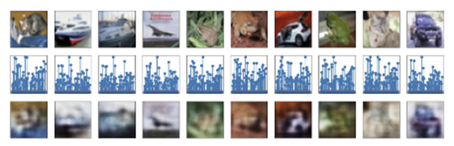
• Q2A. Attach the results of show_ae, where the model was initiated with z_dim=[340, 180] 

• Q2B. Attach the results of show_ae, where the model was initiated with z_dim=[320, 290] 

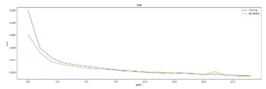
• Q2C. Compare two models and the model in Q1B in terms of reconstruction quality and validation loss, considering the number of tunable parameters 

 

<코드>

from tensorflow.keras import layers, models

class SAE(models.Model):
    def __init__(self, x_nodes=784, z_dim=36):
        x_shape = (x_nodes, )
        x = layers.Input(shape=x_shape)
        h1 = layers.Dense(z_dim[0], activation='relu')(x)
        z = layers.Dense(z_dim[1], activation='relu')(h1)
        h2 = layers.Dense(z_dim[0], activation='relu')(z)
        y = layers.Dense(x_nodes, activation='sigmoid')(h2)

        super().__init__(x, y)
        self.compile(optimizer='adam', loss='mse', metrics=['accuracy'])

        self.x = x
        self.z = z
        self.z_dim = z_dim

    def Encoder(self):
        return models.Model(self.x, self.z)

    def Decoder(self):
        z_shape = (self.z_dim[1], )
        z = layers.Input(shape=z_shape)
        h2_layer = self.layers[-2]
        y_layer = self.layers[-1]
        h2 = h2_layer(z)
        y = y_layer(h2)
        return models.Model(z, y)

from tensorflow.keras.datasets import cifar10
import numpy as np
import matplotlib.pyplot as plt

def plot(history, plot_type, q):
    h = history.history
    path = "./result/"
    val_type = "val_" + plot_type
    plt.plot(h[plot_type])
    plt.plot(h[val_type])
    plt.title(plot_type)
    plt.ylabel(plot_type)
    plt.xlabel("Epoch")
    plt.legend(['Training', 'Validation'], loc=0)
    plt.savefig(path + plot_type + '_' + q + '.jpg')
    plt.clf()

def data_load():
    (x_train, _), (x_test, _) = cifar10.load_data()

    x_train = x_train.astype('float32') / 255
    x_test = x_test.astype('float32') / 255
    x_train = x_train.reshape((len(x_train), np.prod(x_train.shape[1:])))
    x_test = x_test.reshape((len(x_test), np.prod(x_test.shape[1:])))
    return (x_train, x_test)

def show_ae(autoencoder, x_test, qnum):
    path = "./result/show_ae_" + qnum + ".jpg"

    encoder = autoencoder.Encoder()
    decoder = autoencoder.Decoder()
    encoded_imgs = encoder.predict(x_test)
    decoded_imgs = decoder.predict(encoded_imgs)

    n = 10
    plt.figure(figsize=(20, 6))

    for i in range(n):
        ax = plt.subplot(3, n, i+1)
        plt.imshow(x_test[i].reshape(32, 32, 3))
        plt.gray()
        ax.get_xaxis().set_visible(False)
        ax.get_yaxis().set_visible(False)

        ax = plt.subplot(3, n, i+1+n)
        plt.stem(encoded_imgs[i].reshape(-1), use_line_collection=True)
        plt.gray()
        ax.get_xaxis().set_visible(False)
        ax.get_yaxis().set_visible(False)

        ax = plt.subplot(3, n, i + 1 + n + n)
        plt.imshow(decoded_imgs[i].reshape(32, 32, 3))
        plt.gray()
        ax.get_xaxis().set_visible(False)
        ax.get_yaxis().set_visible(False)

    plt.savefig(path)
    plt.clf()

def main():
    """
    q2. Stacked Auto-Encoder
        data_load() : mnist => cifar10          V
        main() : x_nodes = 32 * 32 * 3          V
        AE.__init__() : lossfunction = "mse"    V
        show_ae() : (28, 28) => (32, 32, 3)     V

        a. show_ae() : hidden neurons = 36
        b. show_ae() : hidden neurons = 360
        c. show_ae() : hidden neurons = 1080
    """

    alp = ["Q2a", "Q2b"]
    alpnum = {
        "Q2a" : [340, 180],
        "Q2b" : [340, 290]
    }

    x_nodes = 32 * 32 * 3

    for q in alp:
        qnum = q
        z_dim = alpnum[q]

        (x_train, x_test) = data_load()
        autoencoder = SAE(x_nodes, z_dim)

        history = autoencoder.fit(
            x_train, x_train,
            epochs = 20,
            batch_size = 256,
            shuffle = True,
            validation_data = (x_test, x_test)
        )

        show_ae(autoencoder, x_test, qnum)
        plot(history, "loss", qnum)
        plot(history, "accuracy", qnum)

if __name__ == "__main__":
    main()

Show_ae (z_dim=[340, 180])

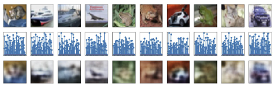
Show_ae (z_dim=[320, 290])

 

SAE를 이용하여 학습시킨 결과 2개와 Q1B의 결과를 비교해보았을 때 먼저 reconstruction quality를 비교해보면 우선 육안으로는 3가지 결과 모두 비슷하게 나온 것을 보인다. 좀 더 꼼꼼히 보면 아주 살짝 다른 점들도 존재는 하지만 3가지 모두 비슷한 결과가 나왔다고 생각한다.

Validation Loss를 비교해보면

Q2A :

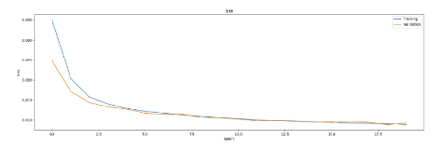
Q2B :

Q1B :

위와 같은 결과의 그래프를 확인할 수 있으며 그래프로 비교를 해보면 AE를 활용한 Q1B가 가장 loss값이 낮게 나온 것 같다.

Tunable parameters를 비교해보면 Q1B는 hidden neuron이 360개이고 Q2A는 340 x 180, Q2B는 320 x 290으로 Q2B가 가장 많아 가장 좋은 결과를 나타냈다고 생각한다.