
printf("ho_tari\n");
PCA #13 본문
<코드>
from tensorflow.keras import layers, models
from tensorflow.keras.datasets import mnist
from tensorflow.keras import backend as K
import numpy as np
import matplotlib.pyplot as plt

def Conv2D(filters, kernel_size, padding="same", activation="relu"):
    return layers.Conv2D(filters, kernel_size, padding=padding, activation=activation)

class SCAE(models.Model):
    def __init__(self, org_shape=(1,28,28)):
        original = layers.Input(shape=org_shape)
        x = Conv2D(4, (3,3))(original)
        x = layers.MaxPooling2D((2,2), padding="same")(x)
        x = Conv2D(8, (3,3))(x)
        x = layers.MaxPooling2D((2,2), padding="same")(x)
        z = Conv2D(1, (7,7))(x)

        y = Conv2D(16, (3,3))(z)
        y = layers.UpSampling2D((2,2))(y)
        y = Conv2D(8, (3,3))(y)
        y = layers.UpSampling2D((2,2))(y)
        y = Conv2D(4, (3,3))(y)
        decoded = Conv2D(1, (3,3), activation="sigmoid")(y)

        super().__init__(original, decoded)
        self.compile(optimizer='adam', loss="binary_crossentropy", metrics=['accuracy'])

        self.x = x
        self.z = z
        self.original = original
        self.summary()


    def Encoder(self):
        return models.Model(self.original, self.z)

    def Decoder(self):
        z_shape = (7,7,1,)
        z = layers.Input(shape=z_shape)
        h = self.layers[-6](z)
        h = self.layers[-5](h)
        h = self.layers[-4](h)
        h = self.layers[-3](h)
        h = self.layers[-2](h)
        h = self.layers[-1](h)
        return models.Model(z, h)

def show_ae(autoencoder, x_test, qnum="0"):
    path = "./result/show_ae_" + qnum + ".jpg"

    encoder = autoencoder.Encoder()
    encoded_imgs = encoder.predict(x_test)
    decoded_imgs = autoencoder.predict(x_test)

    n = 10
    plt.figure(figsize=(20, 6))

    for i in range(n):
        ax = plt.subplot(4, n, i+1)
        plt.imshow(x_test[i].reshape(28, 28))
        plt.gray()
        ax.get_xaxis().set_visible(False)
        ax.get_yaxis().set_visible(False)

        ax = plt.subplot(4, n, i+1+n)
        plt.stem(encoded_imgs[i].reshape(-1), use_line_collection=True)
        plt.gray()
        ax.get_xaxis().set_visible(False)
        ax.get_yaxis().set_visible(False)

        ax = plt.subplot(4, n, i+1+n*2)
        plt.imshow(encoded_imgs[i].reshape(7,7))
        plt.gray()
        ax.get_xaxis().set_visible(False)
        ax.get_yaxis().set_visible(False)

        ax = plt.subplot(4, n, i+1+n*3)
        plt.imshow(decoded_imgs[i].reshape(28, 28))
        plt.gray()
        ax.get_xaxis().set_visible(False)
        ax.get_yaxis().set_visible(False)

    plt.savefig(path)
    plt.clf()

def plot(history, plot_type, q="0"):
    h = history.history
    path = "./result/"
    val_type = "val_" + plot_type
    plt.plot(h[plot_type])
    plt.plot(h[val_type])
    plt.title(plot_type)
    plt.ylabel(plot_type)
    plt.xlabel("Epoch")
    plt.legend(['Training', 'Validation'], loc=0)
    plt.savefig(path + plot_type + '_' + q + '.jpg')
    plt.clf()

def data_load():
    (x_train, _), (x_test, _) = mnist.load_data()

    x_train = x_train.astype('float32') / 255
    x_test = x_test.astype('float32') / 255
    [_, W, H] = x_train.shape
    x_train = x_train.reshape((-1, W, H, 1))
    x_test = x_test.reshape((-1, W, H, 1))
    return (x_train, x_test)

def main(epochs=20, batch_size=128):
    input_shape=[28, 28, 1]
    (x_train, x_test) = data_load()
    autoencoder = SCAE(input_shape)

    history = autoencoder.fit(
        x_train, x_train,
        epochs=epochs,
        batch_size=batch_size,
        shuffle=True,
        validation_data=(x_test, x_test)
    )

    plot(history, "loss")
    plot(history, "accuracy")
    show_ae(autoencoder, x_test)


if __name__ == "__main__":
    main(1)
Q1
• We are going to apply SCAE to cifar10 dataset.
• 1) Change the function data_load (Hint. you don’t need to reshape the dataset.)
• 2) in the function “main” (Hint. you need to update “input_shape”)
• 3) in the function __init__ of class AE (Hint. you also need to update the size of output layer besides the loss function) • 4) in the function “show_ae” (Hint. you also need to update the size of codes.)
• Q1A. Show your updated codes
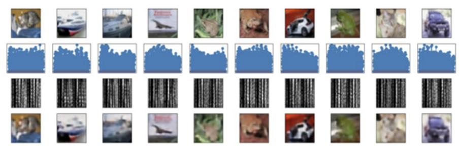
• Q1B. Attach the results of show_ae
<코드>
from tensorflow.keras import layers, models
from tensorflow.keras.datasets import cifar10
import numpy as np
import matplotlib.pyplot as plt

def Conv2D(filters, kernel_size, padding="same", activation="relu"):
    return layers.Conv2D(filters, kernel_size, padding=padding, activation=activation)

class SCAE(models.Model):
    def __init__(self, org_shape=(3,32,32)):
        original = layers.Input(shape=org_shape)
        x = Conv2D(4, (3,3))(original)
        x = layers.MaxPooling2D((2,2), padding="same")(x)
        x = Conv2D(8, (3,3))(x)
        x = layers.MaxPooling2D((2,2), padding="same")(x)
        z = Conv2D(1, (7,7))(x)

        y = Conv2D(16, (3,3))(z)
        y = layers.UpSampling2D((2,2))(y)
        y = Conv2D(8, (3,3))(y)
        y = layers.UpSampling2D((2,2))(y)
        y = Conv2D(4, (3,3))(y)
        decoded = Conv2D(3, (3,3), activation="sigmoid")(y)

        super().__init__(original, decoded)
        self.compile(optimizer='adam', loss="mse", metrics=['accuracy'])

        self.x = x
        self.z = z
        self.original = original
        self.summary()


    def Encoder(self):
        return models.Model(self.original, self.z)

    def Decoder(self):
        z_shape = (8,8,1,)
        z = layers.Input(shape=z_shape)
        h = self.layers[-6](z)
        h = self.layers[-5](h)
        h = self.layers[-4](h)
        h = self.layers[-3](h)
        h = self.layers[-2](h)
        h = self.layers[-1](h)
        return models.Model(z, h)

def show_ae(autoencoder, x_test, qnum="1"):
    path = "./result/show_ae_" + qnum + ".jpg"

    encoder = autoencoder.Encoder()
    encoded_imgs = encoder.predict(x_test)
    decoded_imgs = autoencoder.predict(x_test)

    n = 10
    plt.figure(figsize=(20, 6))

    for i in range(n):
        ax = plt.subplot(4, n, i+1)
        plt.imshow(x_test[i].reshape(32, 32, 3))
        plt.gray()
        ax.get_xaxis().set_visible(False)
        ax.get_yaxis().set_visible(False)

        ax = plt.subplot(4, n, i+1+n)
        plt.stem(encoded_imgs[i].reshape(-1), use_line_collection=True)
        plt.gray()
        ax.get_xaxis().set_visible(False)
        ax.get_yaxis().set_visible(False)

        ax = plt.subplot(4, n, i+1+n*2)
        plt.imshow(encoded_imgs[i].reshape(8,8))
        plt.gray()
        ax.get_xaxis().set_visible(False)
        ax.get_yaxis().set_visible(False)

        ax = plt.subplot(4, n, i+1+n*3)
        plt.imshow(decoded_imgs[i].reshape(32, 32, 3))
        plt.gray()
        ax.get_xaxis().set_visible(False)
        ax.get_yaxis().set_visible(False)

    plt.savefig(path)
    plt.clf()

def plot(history, plot_type, q="1"):
    h = history.history
    path = "./result/"
    val_type = "val_" + plot_type
    plt.plot(h[plot_type])
    plt.plot(h[val_type])
    plt.title(plot_type)
    plt.ylabel(plot_type)
    plt.xlabel("Epoch")
    plt.legend(['Training', 'Validation'], loc=0)
    plt.savefig(path + plot_type + '_' + q + '.jpg')
    plt.clf()

def data_load():
    (x_train, _), (x_test, _) = cifar10.load_data()

    x_train = x_train.astype('float32') / 255
    x_test = x_test.astype('float32') / 255
    [_, W, H, _] = x_train.shape
    # x_train = x_train.reshape((-1, W, H, 1))
    # x_test = x_test.reshape((-1, W, H, 1))
    return (x_train, x_test)

def main(epochs=20, batch_size=128):
    input_shape=[32, 32, 3]
    (x_train, x_test) = data_load()
    autoencoder = SCAE(input_shape)

    history = autoencoder.fit(
        x_train, x_train,
        epochs=epochs,
        batch_size=batch_size,
        shuffle=True,
        validation_data=(x_test, x_test)
    )

    plot(history, "loss")
    plot(history, "accuracy")
    show_ae(autoencoder, x_test)


if __name__ == "__main__":
    main(1)
Show_ae

Q2
• The results of the previous SCAE model (Q1B) were not good enough.
• There are two different ways of improvement.
• A. Increased the number of filters.
• B. increased the size of codes.
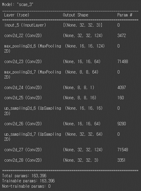
• Q2A. Change the number of filters as follows, and attach the results of show_ae.
124, 64, 1, 16, 64, 124
• Q2B. Change the number of filters as follows, and attach the results of show_ae.
82, 64, 16, 16, 64, 82
• Q2C. Compare two models (Q2A and Q2B) in terms of reconstruction quality and validation loss, considering the number of tunable parameters
<Q2A 코드>
from tensorflow.keras import layers, models
from tensorflow.keras.datasets import cifar10

def Conv2D(filters, kernel_size, padding="same", activation="relu"):
    return layers.Conv2D(filters, kernel_size, padding=padding, activation=activation)

class SCAE(models.Model):
    def __init__(self, org_shape=(3,32,32)):
        original = layers.Input(shape=org_shape)
        x = Conv2D(124, (3,3))(original)
        x = layers.MaxPooling2D((2,2), padding="same")(x)
        x = Conv2D(64, (3,3))(x)
        x = layers.MaxPooling2D((2,2), padding="same")(x)
        z = Conv2D(1, (7,7))(x)

        y = Conv2D(16, (3,3))(z)
        y = layers.UpSampling2D((2,2))(y)
        y = Conv2D(64, (3,3))(y)
        y = layers.UpSampling2D((2,2))(y)
        y = Conv2D(124, (3,3))(y)
        decoded = Conv2D(3, (3,3), activation="sigmoid")(y)

        super().__init__(original, decoded)
        self.compile(optimizer='adam', loss="mse", metrics=['accuracy'])

        self.x = x
        self.z = z
        self.original = original
        self.summary()

    def Encoder(self):
        return models.Model(self.original, self.z)

    def Decoder(self):
        z_shape = (8,8)
        z = layers.Input(shape=z_shape)
        h = self.layers[-6](z)
        h = self.layers[-5](h)
        h = self.layers[-4](h)
        h = self.layers[-3](h)
        h = self.layers[-2](h)
        h = self.layers[-1](h)
        return models.Model(z, h)

from tensorflow.keras.datasets import cifar10
import numpy as np
import matplotlib.pyplot as plt

def plot(history, plot_type, q="2A"):
    h = history.history
    path = "./result/"
    val_type = "val_" + plot_type
    plt.plot(h[plot_type])
    plt.plot(h[val_type])
    plt.title(plot_type)
    plt.ylabel(plot_type)
    plt.xlabel("Epoch")
    plt.legend(['Training', 'Validation'], loc=0)
    plt.savefig(path + plot_type + '_' + q + '.jpg')
    plt.clf()

def data_load():
    (x_train, _), (x_test, _) = cifar10.load_data()

    x_train = x_train.astype('float32') / 255
    x_test = x_test.astype('float32') / 255
    [_, W, H, _] = x_train.shape
    # x_train = x_train.reshape((-1, W, H, 1))
    # x_test = x_test.reshape((-1, W, H, 1))
    return (x_train, x_test)

def show_ae(autoencoder, x_test, qnum="2A"):
    path = "./result/show_ae_" + qnum + ".jpg"

    encoder = autoencoder.Encoder()
    encoded_imgs = encoder.predict(x_test)
    decoded_imgs = autoencoder.predict(x_test)

    n = 10
    plt.figure(figsize=(20, 6))

    for i in range(n):
        ax = plt.subplot(4, n, i+1)
        plt.imshow(x_test[i].reshape(32, 32, 3))
        plt.gray()
        ax.get_xaxis().set_visible(False)
        ax.get_yaxis().set_visible(False)

        ax = plt.subplot(4, n, i+1+n)
        plt.stem(encoded_imgs[i].reshape(-1), use_line_collection=True)
        plt.gray()
        ax.get_xaxis().set_visible(False)
        ax.get_yaxis().set_visible(False)

        ax = plt.subplot(4, n, i+1+n*2)
        plt.imshow(encoded_imgs[i].reshape(8, 8))
        plt.gray()
        ax.get_xaxis().set_visible(False)
        ax.get_yaxis().set_visible(False)

        ax = plt.subplot(4, n, i+1+n*3)
        plt.imshow(decoded_imgs[i].reshape(32, 32, 3))
        plt.gray()
        ax.get_xaxis().set_visible(False)
        ax.get_yaxis().set_visible(False)

    plt.savefig(path)
    plt.clf()

def main(epochs=20, batch_size=128):
    input_shape=[32, 32, 3]
    (x_train, x_test) = data_load()
    autoencoder = SCAE(input_shape)

    history = autoencoder.fit(
        x_train, x_train,
        epochs=epochs,
        batch_size=batch_size,
        shuffle=True,
        validation_data=(x_test, x_test)
    )

    plot(history, "loss")
    plot(history, "accuracy")
    show_ae(autoencoder, x_test)


if __name__ == "__main__":
    main(1)
<Q2B 코드>
from tensorflow.keras import layers, models
from tensorflow.keras.datasets import cifar10

def Conv2D(filters, kernel_size, padding="same", activation="relu"):
    return layers.Conv2D(filters, kernel_size, padding=padding, activation=activation)

class SCAE(models.Model):
    def __init__(self, org_shape=(3,32,32)):
        original = layers.Input(shape=org_shape)
        x = Conv2D(82, (3,3))(original)
        x = layers.MaxPooling2D((2,2), padding="same")(x)
        x = Conv2D(64, (3,3))(x)
        x = layers.MaxPooling2D((2,2), padding="same")(x)
        z = Conv2D(16, (7,7))(x)

        y = Conv2D(16, (3,3))(z)
        y = layers.UpSampling2D((2,2))(y)
        y = Conv2D(64, (3,3))(y)
        y = layers.UpSampling2D((2,2))(y)
        y = Conv2D(82, (3,3))(y)
        decoded = Conv2D(3, (3,3), activation="sigmoid")(y)

        super().__init__(original, decoded)
        self.compile(optimizer='adam', loss="mse", metrics=['accuracy'])

        self.x = x
        self.z = z
        self.original = original
        self.summary()

    def Encoder(self):
        return models.Model(self.original, self.z)

    def Decoder(self):
        z_shape = (8,8,16)
        z = layers.Input(shape=z_shape)
        h = self.layers[-6](z)
        h = self.layers[-5](h)
        h = self.layers[-4](h)
        h = self.layers[-3](h)
        h = self.layers[-2](h)
        h = self.layers[-1](h)
        return models.Model(z, h)

from tensorflow.keras.datasets import cifar10
import numpy as np
import matplotlib.pyplot as plt

def plot(history, plot_type, q="2B"):
    h = history.history
    path = "./result/"
    val_type = "val_" + plot_type
    plt.plot(h[plot_type])
    plt.plot(h[val_type])
    plt.title(plot_type)
    plt.ylabel(plot_type)
    plt.xlabel("Epoch")
    plt.legend(['Training', 'Validation'], loc=0)
    plt.savefig(path + plot_type + '_' + q + '.jpg')
    plt.clf()

def data_load():
    (x_train, _), (x_test, _) = cifar10.load_data()

    x_train = x_train.astype('float32') / 255
    x_test = x_test.astype('float32') / 255
    [_, W, H, _] = x_train.shape
    # x_train = x_train.reshape((-1, W, H, 1))
    # x_test = x_test.reshape((-1, W, H, 1))
    return (x_train, x_test)

def show_ae(autoencoder, x_test, qnum="2B"):
    path = "./result/show_ae_" + qnum + ".jpg"

    encoder = autoencoder.Encoder()
    encoded_imgs = encoder.predict(x_test)
    decoded_imgs = autoencoder.predict(x_test)

    n = 10
    plt.figure(figsize=(20, 6))

    for i in range(n):
        ax = plt.subplot(4, n, i+1)
        plt.imshow(x_test[i].reshape(32, 32, 3))
        plt.gray()
        ax.get_xaxis().set_visible(False)
        ax.get_yaxis().set_visible(False)

        ax = plt.subplot(4, n, i+1+n)
        plt.stem(encoded_imgs[i].reshape(-1), use_line_collection=True)
        plt.gray()
        ax.get_xaxis().set_visible(False)
        ax.get_yaxis().set_visible(False)

        ax = plt.subplot(4, n, i+1+n*2)
        plt.imshow(encoded_imgs[i].reshape(8, 8))
        plt.gray()
        ax.get_xaxis().set_visible(False)
        ax.get_yaxis().set_visible(False)

        ax = plt.subplot(4, n, i+1+n*3)
        plt.imshow(decoded_imgs[i].reshape(32, 32, 3))
        plt.gray()
        ax.get_xaxis().set_visible(False)
        ax.get_yaxis().set_visible(False)

    plt.savefig(path)
    plt.clf()

def main(epochs=20, batch_size=128):
    input_shape=[32, 32, 3]
    (x_train, x_test) = data_load()
    autoencoder = SCAE(input_shape)

    history = autoencoder.fit(
        x_train, x_train,
        epochs=epochs,
        batch_size=batch_size,
        shuffle=True,
        validation_data=(x_test, x_test)
    )

    plot(history, "loss")
    plot(history, "accuracy")
    show_ae(autoencoder, x_test)


if __name__ == "__main__":
    main()
Show_ae (case 1)

Show_ae (case 2)
Q2A의 summary :
Q2B의 summary :
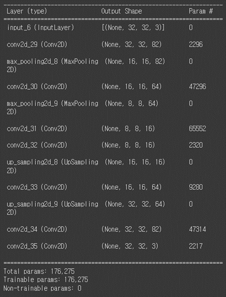
Filter의 개수를 증가시킨 (a)의 경우에는 validation loss 가 0.0130이고, Code의 사이즈를 증가시킨 (b)의 경우에는 validation loss 가 0.0028이 나왔다. Model Summary를 통해 parameter의 개수를 확인해본 결과, (a)의 경우에는 163,396개, (b)의 경우에는 176,275개이다. Parameter의 수는 (a)의 경우가 더 적지만 loss 값이 더 크게 나온 바를 보면 code의 사이즈를 증가시킨 경우가 더 성능이 좋다고 판단할 수 있다. 실제로 위에 첨부한 ae 사진을 확인하면 단순히 필터의 개수를 늘린 (a)의 경우보다 (b)의 경우가 원래 True 값과 더 유사하게 출력되었음을 알 수 있다.
Q3
• Implement the code of U-net for simple reconstruction of CIFAR10 on the slides 7-16.
• Set the following learning parameters: Batch_size=128, Epochs=200
• Change the number of filters in order: 56, 32, 16, 32, 56
• Q3A. How many does the model has as its total parameters? (See model.summary())
• Q3B. Attach the predictions (bottom figures on the slide 17)
• Q3C. Compare the result with that of Q2B, in terms of loss and quality of reconstruction
<코드>
from tensorflow.keras import layers, models
from tensorflow.keras.datasets import cifar10

import matplotlib.pyplot as plt

class Unet(models.Model):
    def conv(x, n_f, mp_flag=True):
        if mp_flag:
            x = layers.MaxPooling2D((2,2), padding="same")(x)
        x = layers.Conv2D(n_f, (3,3), padding="same")(x)
        x = layers.BatchNormalization()(x)
        x = layers.Activation("tanh")(x)
        x = layers.Dropout(0.05)(x)
        x = layers.Conv2D(n_f, (3,3), padding="same")(x)
        x = layers.BatchNormalization()(x)
        x = layers.Activation("tanh")(x)
        return x

    def deconv_unet(x, e, n_f):
        x = layers.UpSampling2D((2,2))(x)
        x = layers.Concatenate(axis=3)([x, e]) ##*****
        x = layers.Conv2D(n_f, (3,3), padding="same")(x)
        x = layers.BatchNormalization()(x)
        x = layers.Activation("tanh")(x)
        x = layers.Conv2D(n_f, (3,3), padding="same")(x)
        x = layers.BatchNormalization()(x)
        x = layers.Activation("tanh")(x)
        return x

    def __init__(self, org_shape):
        original = layers.Input(shape=org_shape)

        c1 = Unet.conv(original, 16, mp_flag=False)
        c2 = Unet.conv(c1, 32)

        encoded = Unet.conv(c2, 64)

        x = Unet.deconv_unet(encoded, c2, 32)
        y = Unet.deconv_unet(x, c1, 16)

        decoded = layers.Conv2D(3, (3,3), activation="sigmoid", padding="same")(y)

        super().__init__(original, decoded)
        self.compile(optimizer="adadelta", loss="mse")

class Data():
    def __init__(self):
        (x_train, y_train), (x_test, y_test) = cifar10.load_data()
        x_train = x_train.astype("float32")/255
        x_test = x_test.astype("float32")/255

        self.x_train_in = x_train
        self.x_test_in = x_test
        self.x_train_out = x_train
        self.x_test_out = x_test

        img_rows, img_cols, n_ch = self.x_train_in.shape[1:]
        self.input_shape = (img_rows, img_cols, n_ch)

def show_images(data, unet):
    x_test_in = data.x_test_in
    x_test_out = data.x_test_out
    decoded_imgs = unet.predict(x_test_in)

    n = 10
    plt.figure(figsize=(20, 6))

    for i in range(n):
        ax = plt.subplot(3, n, i+1)
        plt.imshow(x_test_in[i])
        ax.get_xaxis().set_visible(False)
        ax.get_yaxis().set_visible(False)

        ax = plt.subplot(3, n, i+1+n)
        plt.imshow(decoded_imgs[i])
        ax.get_xaxis().set_visible(False)
        ax.get_yaxis().set_visible(False)

        ax = plt.subplot(3, n, i+1+n*2)
        plt.imshow(x_test_out[i])
        ax.get_xaxis().set_visible(False)
        ax.get_yaxis().set_visible(False)

    plt.savefig("show_images_Q3.jpg")
    plt.clf()

def plot_loss(history):
    h = history.history
    plt.plot(history["loss"])
    plt.plot(history["val_loss"])
    plt.xlabel("Epochs")
    plt.ylabel("Loss")
    plt.legend(["loss", "val_loss"])
    plt.title("Loss")
    plt.savefig("loss_graph_Q3.jpg")
    plt.clf()


def main(epochs=10, batch_size=512, fig=True):
    data = Data()
    unet = Unet(data.input_shape)
    unet.summary()

    history = unet.fit(
        data.x_train_in, data.x_train_out,
        epohcs = epochs, batch_size = batch_size,
        shuffle = True,
        validation_data = (data.x_test_in, data.x_test_out)
    )

    if fig:
        plot_loss(history)
        show_images(data, unet)

if __name__ == "__main__":
    main()
Q3A
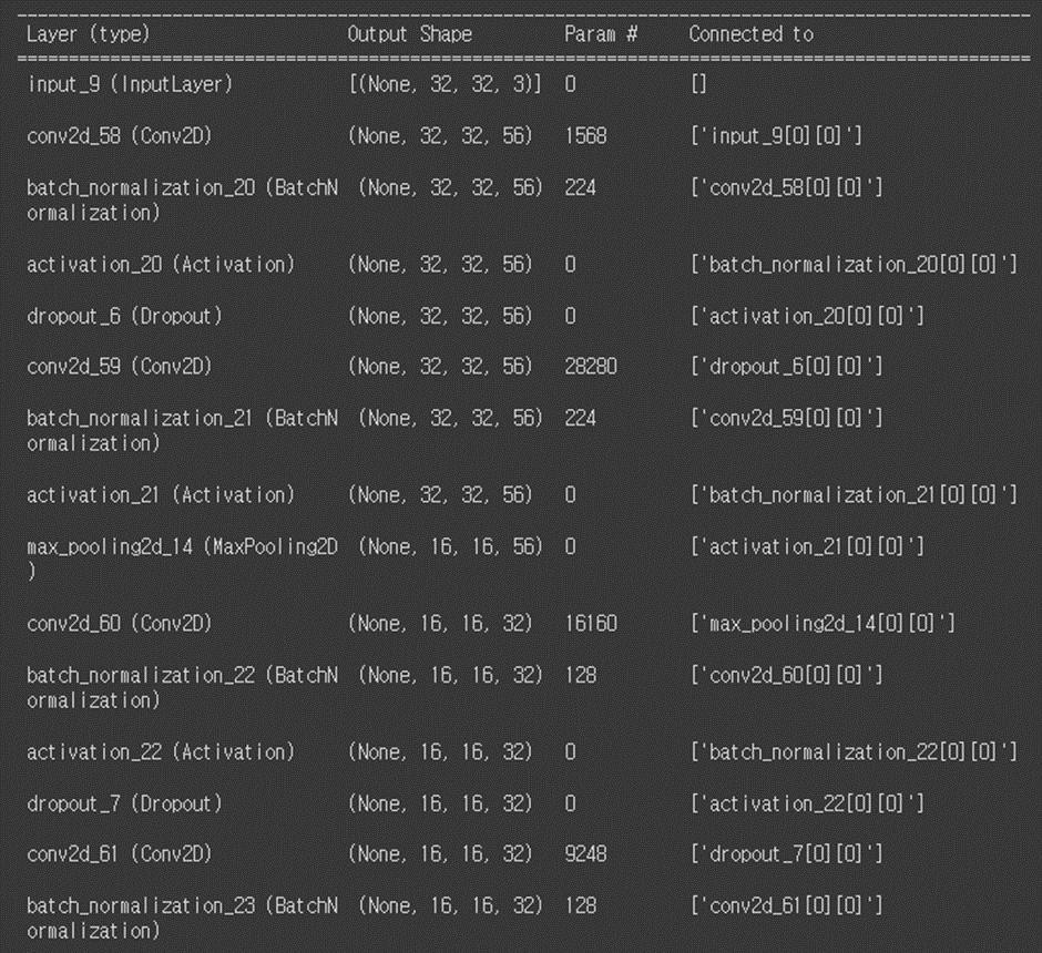

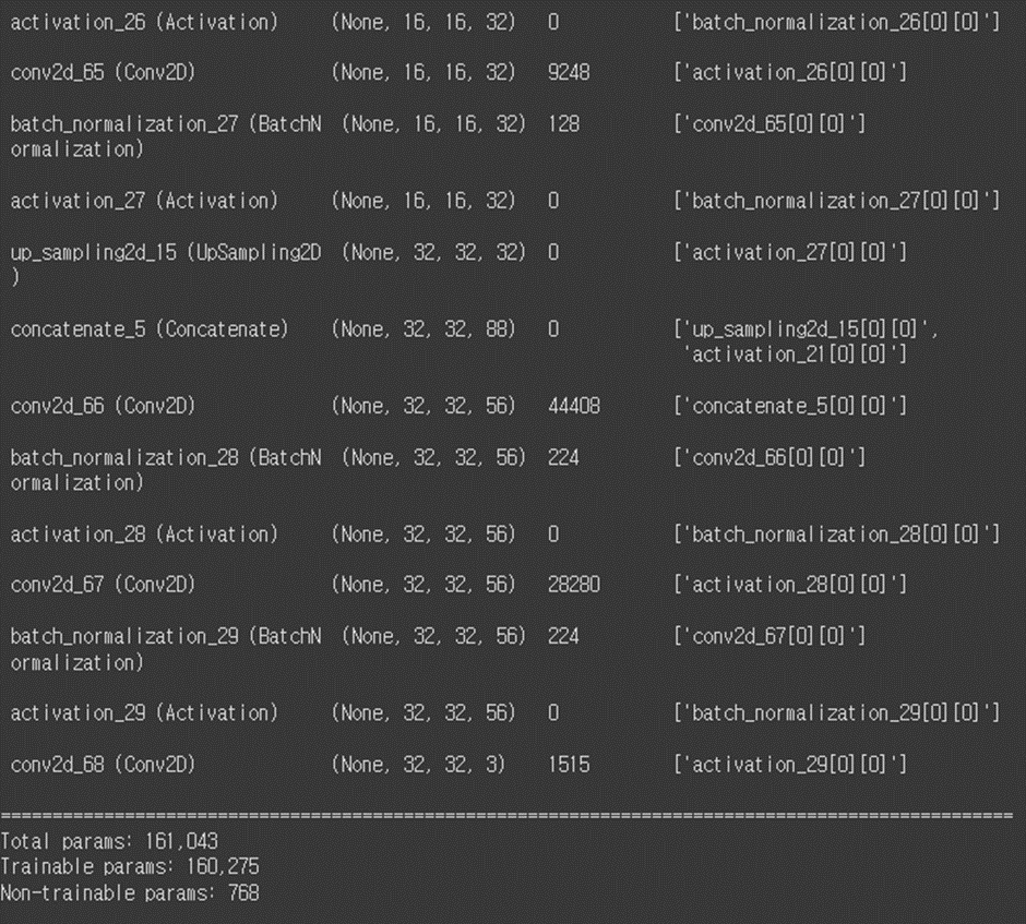
Toral parameters: 161,043개
Trainable parameters: 160,275개
Non-trainable parameters: 768개
Q3B
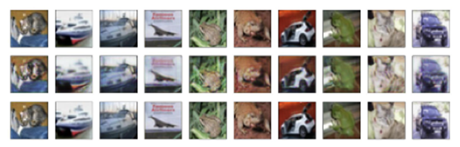
Q3C
Q2B에서 SCAE를 이용하고 code의 사이즈를 증가시킨 경우의 loss 값은 0.0028이었다. Q3의 경우에는 UNET을 사용한 경우에는 loss 값이 0.0047이었다. UNET을 사용한 경우에 적은 parameter 로 더 큰 loss 값이 나왔다. UNET의 loss값이 더 크게 나왔지만 skip connection에 의해 image의 선명도는 더 잘 나온 것을 알 수 있어 Q3의 결과가 더 좋다고 생각한다. 또한, 실제 이미지가 출력된 것을 보면 UNET의 경우 예측이 잘 되었다.


