
printf("ho_tari\n");
ep.40 퍼셉트론, 신경망 본문
2024.9.2
퍼셉트론(Perceptron)
다수의 신호를 입력으로 받아 하나의 신호를 출력한다.
신호 : 전류나 강물처럼 흐름이 있는 것
전류가 전선을 타고 흐르는 전자를 보내듯, 퍼셉트론 신호도 흐름을 말들고 정보를 앞으로 전달
실제 전류와 달리 퍼셉트론 신호는 흐른다/안 흐른다(1이나 0)의 두가지 값을 가질 수 있다.
- 1 : 신호가 흐른다.
- 0 : 신호가 흐르지 않는다.


입력으로 두개의 신호를 받은 퍼셉트론의 예
- x1과 x2는 입력신호
- y는 출력신호
- w1과 w2는 가중치
- 그림의 원을 뉴런 혹은 노드라고 부른다.
- 입력신호가 뉴런에 보내질 때는 각각 고유의 가중치가 곱해진다.(w1x1 + w2x2)
- 뉴런에서 보내온 신호의 총합이 정해진 한계를 넘어설 때만 1을 출력
- 한계를 임계값이라한다.
가중치는 각 신호가 결과에 주는 영향력을 조절하는 요소
가중치가 클 수록 결과에 주는 영향이 크다.
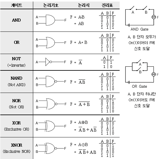
단순한 논리 회로
AND 게이트 진리표

NAND 게이트 진리표

OR 게이트 진리표

- 각 Gate 별 진리표를 구한다.
- 각각의 Gate는 퍼셉트론으로 구현이 가능한다.
논리회로 진리표

- AND 함수 : w1, w2, theta 사용 구현
def AND(x1, x2):
    w1, w2, theta = 0.5, 0.5, 0.7       # and
    #w1, w2, theta = 0.5, 0.5, 0.2       # or
    #w1, w2, theta = -0.5, -0.5, -0.2    # nor
    #w1, w2, theta = -0.5, -0.5, -0.7    # nand
    tmp = x1 * w1 + x2 * w2
    if tmp <= theta:
        return 0
    elif tmp > theta:
        return 1

print(AND(0, 0))
print(AND(0, 1))
print(AND(1, 0))
print(AND(1, 1))
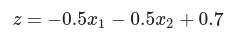
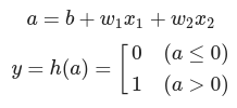
가중치와 편향 도입


퍼셉트론의 파라미터(w1, w2, b)를 조정하여 논리회로를 구현함
AND gate
(w1, w2, b) = (0.5, 0.5, -0.7)일 때
AND 게이트 퍼셉트론 식
가중치(w1, w2)와 편향(b)

activation function

SCALAR 연산
def AND(x1, x2):
    w1, w2, b = 0.5, 0.5, -0.7       # and
    tmp = x1 * w1 + x2 * w2 + b
    if tmp <= 0:
        return 0
    elif tmp > 0:
        return 1

if __name__ == '__main__':
    for xs in [(0, 0), (1, 0), (0, 1), (1, 1)]:
        y = AND(xs[0], xs[1])
        print(str(xs) + " -> " + str(y))
VECTOR 연산
# coding: utf-8
import numpy as np

def AND(x1, x2):
    x = np.array([x1, x2])
    w = np.array([0.5, 0.5])
    b = -0.7
    tmp = np.sum(w*x) + b
    if tmp <= 0:
        return 0
    else:
        return 1

for xs in [(0, 0), (1, 0), (0, 1), (1, 1)]:
    y = AND(xs[0], xs[1])
    print(str(xs) + " -> " + str(y))
OR gate
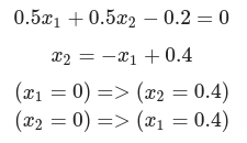
(w1, w2, b) = (0.5, 0.5, -0.2)일 때
OR 게이트 퍼셉트론 식
가중치(w1, w2)와 편향(b)

activation function

# or_gate.py
# coding: utf-8
import numpy as np

def OR(x1, x2):
    x = np.array([x1, x2])
    w = np.array([0.5, 0.5])
    b = -0.2
    tmp = np.sum(w*x) + b
    if tmp <= 0:
        return 0
    else:
        return 1

if __name__ == '__main__':
    for xs in [(0, 0), (1, 0), (0, 1), (1, 1)]:
        y = OR(xs[0], xs[1])
        print(str(xs) + " -> " + str(y))
NAND gate
(w1, w2, b) = (-0.5, -0.5, 0.7)일 때
NAND 게이트 퍼셉트론 식
가중치(w1, w2)와 편향(b)
activation function

# nand_gate.py
# coding: utf-8
import numpy as np

def NAND(x1, x2):
    x = np.array([x1, x2])
    w = np.array([-0.5, -0.5])
    b = 0.7
#    b = 0.5
    tmp = np.sum(w*x) + b
    if tmp <= 0:
        return 0
    else:
        return 1

if __name__ == '__main__':
    for xs in [(0, 0), (1, 0), (0, 1), (1, 1)]:
        y = NAND(xs[0], xs[1])
        print(str(xs) + " -> " + str(y))
바이어스에 따른 논리회로의 변화
AND 와 OR
# coding: utf-8
import numpy as np


def AND(x1, x2):
    x = np.array([x1, x2])
    w = np.array([0.5, 0.5])
    #b = -1.0   # all 0
    #b = -0.9   # and
    #b = -0.8   # and
    #b = -0.7   # and original
    #b = -0.6   # and
    #b = -0.5   # and
    #b = -0.4   # or
    #b = -0.3   # or
    #b = -0.2   # or
    #b = -0.1   # or
    #b =  0.0   # or
    b =  0.1   # all 1
    tmp = np.sum(w*x) + b
    if tmp <= 0:
        return 0
    else:
        return 1

if __name__ == '__main__':
    for xs in [(0, 0), (1, 0), (0, 1), (1, 1)]:
        y = AND(xs[0], xs[1])
        print(str(xs) + " -> " + str(y))
NAND 와 NOR
# coding: utf-8
import numpy as np

def NAND(x1, x2):
    x = np.array([x1, x2])
    w = np.array([-0.5, -0.5])
    #b =  1.2   # all 1
    #b =  1.1   # all 1
    #b =  1.0   # nand
    #b =  0.9   # nand
    #b =  0.8   # nand
    b =  0.7   # nand original
    #b =  0.6   # nand
    #b =  0.5   # nor
    #b =  0.4   # nor
    #b =  0.3   # nor
    #b =  0.2   # nor
    #b =  0.1   # nor
    #b = -0.0   # all 0
    #b = -0.1   # all 0
    tmp = np.sum(w*x) + b
    if tmp <= 0:
        return 0
    else:
        return 1

if __name__ == '__main__':
    for xs in [(0, 0), (1, 0), (0, 1), (1, 1)]:
        y = NAND(xs[0], xs[1])
        print(str(xs) + " -> " + str(y))
퍼셉트론의 한계
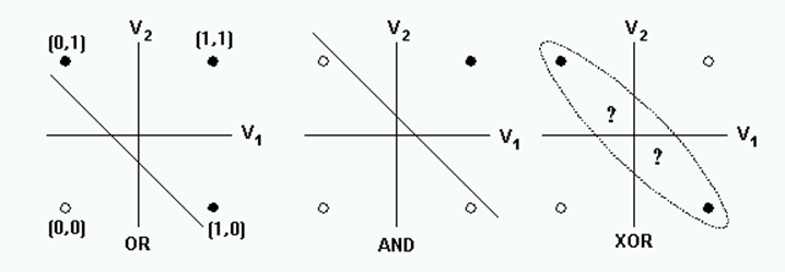
- 증명
다층 퍼셉트론


# coding: utf-8
def XOR(x1, x2):
    s1 = NAND(x1, x2)
    s2 = OR(x1, x2)

    y = AND(s1, s2)
    return y

if __name__ == '__main__':
    for xs in [(0, 0), (1, 0), (0, 1), (1, 1)]:
        y = XOR(xs[0], xs[1])
        print(str(xs) + " -> " + str(y))
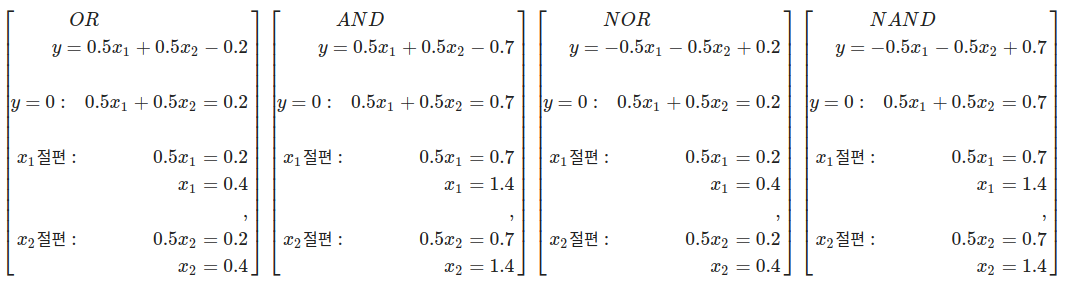
OR
%matplotlib inline

import numpy as np
import matplotlib.pyplot as plt
import matplotlib

x1 = np.arange(-0.1, 1.1, 0.7)
x2 = -x1 + 0.4

plt.axvline(x=0, color = 'b')  # draw x =0 axes
plt.axhline(y=0, color = 'b')   # draw y =0 axes

# 그래프 그리기
plt.plot(x1, x2, label="or")
plt.xlabel("X1") # x축 이름
plt.ylabel("X2") # y축 이름
plt.legend()

#plt.fill_between(x1, x2, '-3', color='grey', alpha='0.5')
plt.fill_between(x1, x2, -0.2, color='grey', alpha=0.5)

plt.scatter([0],[0],marker='o',color='r')
plt.scatter([1,0,1],[0,1,1],marker='^',color='r')
plt.show()
AND
%matplotlib inline

import numpy as np
import matplotlib.pyplot as plt
import matplotlib

#x1 = np.arange(-0.1, 1.1, 1)
#x2 = -x1 + 0.4
x1 = np.arange(-0.1, 1.3, 0.2)
x2 = -x1 + 1.4

plt.axvline(x=0, color = 'b')  # draw x =0 axes
plt.axhline(y=0, color = 'b')   # draw y =0 axes

# 그래프 그리기
#plt.plot(x1, x2, label="or")
plt.plot(x1, x2, label="and")
plt.xlabel("X1") # x축 이름
plt.ylabel("X2") # y축 이름
plt.legend()

#plt.fill_between(x1, x2, '-3', color='grey', alpha='0.5')
plt.fill_between(x1, x2, -0.4, color='grey', alpha=0.5)

#plt.scatter([0],[0],marker='o',color='r')
#plt.scatter([1,0,1],[0,1,1],marker='^',color='r')
plt.scatter([0,1,0],[0,0,1],marker='o',color='r')
plt.scatter([1],[1],marker='^',color='r')

plt.show()
NOR
%matplotlib inline

import numpy as np
import matplotlib.pyplot as plt
import matplotlib

x1 = np.arange(-0.1, 1.1, 0.7)
x2 = -x1 + 0.4

plt.axvline(x=0, color = 'b')   # draw x =0 axes
plt.axhline(y=0, color = 'b')   # draw y =0 axes

# 그래프 그리기
plt.plot(x1, x2, label="nor")
plt.xlabel("X1") # x축 이름
plt.ylabel("X2") # y축 이름
plt.legend()

#plt.fill_between(x1, x2, '-3', color='grey', alpha='0.5')
plt.fill_between(x1, x2, -0.2, color='grey', alpha=0.5)

#plt.scatter([0],[0],marker='o',color='r')
#plt.scatter([1,0,1],[0,1,1],marker='^',color='r')
plt.scatter([1,0,1],[0,1,1],marker='o',color='r')
plt.scatter([0],[0],marker='^',color='r')
plt.show()
NAND
%matplotlib inline

import numpy as np
import matplotlib.pyplot as plt
import matplotlib

#x1 = np.arange(-0.1, 1.1, 1)
#x2 = -x1 + 0.4
x1 = np.arange(-0.1, 1.3, 0.2)
x2 = -x1 + 1.4

plt.axvline(x=0, color = 'b')  # draw x =0 axes
plt.axhline(y=0, color = 'b')  # draw y =0 axes

# 그래프 그리기
#plt.plot(x1, x2, label="or")
plt.plot(x1, x2, label="nand")
plt.xlabel("X1") # x축 이름
plt.ylabel("X2") # y축 이름
plt.legend()

#plt.fill_between(x1, x2, '-3', color='grey', alpha='0.5')
plt.fill_between(x1, x2, -0.4, color='grey', alpha=0.5)

#plt.scatter([0],[0],marker='o',color='r')
#plt.scatter([1,0,1],[0,1,1],marker='^',color='r')
plt.scatter([0,1,0],[0,0,1],marker='^',color='r')
plt.scatter([1],[1],marker='o',color='r')

plt.show()
Vector 연산
신경망
- 퍼셉트론으로 복잡한 함수 표현
- 가중치를 설정하는 작업은 사람이 수동으로 처리한다.
퍼셉트론에서 신경망으로
차이 : 퍼셉트론 - 스텝함수, 신경망 - sigmoid 함수 사용
퍼셉트론 장점
- 복잡한 함수도 표현할 수 있다는 것
퍼셉트론 단점
- 가중치 작업하는 작업이 수동으로 진행(Back propagation 이 적용되지 않음)
신경망은 가중치를 자동으로 설정
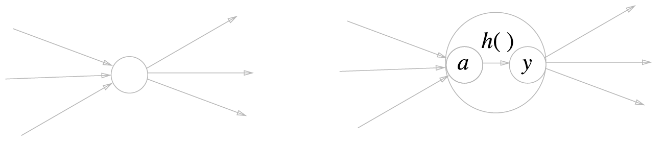
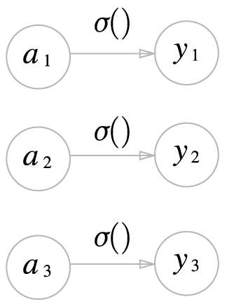
활성화 함수의 등장
활성화 함수의 처리 과정 - 2단계 처리 과정
- a : 가중치가 곱해진 입력신호의 총합
- y : 그합을 활성화 함수(h())에 입력


- a : 가중치가 달린 입력 신호와 편향의 총합
- a를 함수 h()에 넣어 y를 출력
왼쪽은 일반적인 뉴런, 오른쪽은 활성화 처리 과정을 명시한 뉴런(a는 입력 신호의 총합, h()는 활성화 함수, y는 출력)
- 뉴런을 하나의 원으로 그린다. 하나의 노드 임
- a와 y도 하나의 원 즉 노드이다.

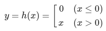
활성화 함수
- 퍼셉트론 : 계단함수
- 신경망 : sigmoid 함수.
계단 함수 구현하기
Step function
import numpy as np
import matplotlib.pylab as plt

def step_function(x):
  if x>0:
    return 1
  else:
    return 0

#numpy 배열을 받기 위한 step function
def step_function(x):
  y = x>0
  return y.astype(np.int)

#numpy용 step_function에서 y.astype(np.int)를 사용하는 이유
x = np.array([-1.0,1.0,2.0])
print(x)

y = x>0
print(y) #y는 bool type

print(y.astype(np.int)) #astype(np.int)를 통해 int형으로 형 변환
계단 함수 그래프
Step function Graph

x = np.arange(-5.0,5.0,0.1)
y = step_function(x)
plt.plot(x,y)
plt.ylim(-0.1,1.1)
plt.show()
시그모이드 함수 구현하기
Sigmoid

def sigmoid(x):
  return 1/(1+np.exp(-x))

x = np.array([-1.0,1.0,2.0])
sigmoid(x)
Sigmoid Graph
x = np.arange(-5.0,5.0,0.1)
print(len(x))
y = sigmoid(x)
plt.plot(x,y)
plt.ylim(-0.1,1.1)
plt.show()
시그모이드 함수와 계단 함수 비교
Sigmoid/Step function 비교
x = np.arange(-5.0, 5.0, 0.1)

y1 = sigmoid(x)
y2 = step_function(x)

plt.plot(x, y1)
plt.plot(x, y2, 'k--')
#plt.plot(x,0.1*x+0.5)
plt.ylim(-0.1, 1.1) # y축 범위 지정
plt.show()
비선형 함수
선형함수만 이용하면 신경망의 층을 깊게하는 의미가 없어지지 때문입니다.
ReLU 함수
def relu(x):
  return np.maximum(0,x)    # 0과 x를 비교하여 최대값 반환. 즉 음수면 0, 양수면 x 반환
ReLU Graph
x = np.arange(-5.0,5.0,0.1)
y = relu(x)
plt.plot(x,y)
plt.ylim(-1.0,5.5)
plt.show()
STEP 함수(활성함수)에 Weight SUM 적용하기
def step_function_withwb(w,x,b):
  y = (w*x+b)>0
  return y.astype(np.int)

# W에 의한 스텝 함수 출력 - 스텝 기울기에 영향을 미치지 않음
x = np.arange(-10.0,10.0,0.1)          # 입력 -10 ~ 10사이의 x값 간격 0.1

y = step_function_withwb(1, x, 0)      # 파란색 W=1
plt.plot(x,y)                          # x 값에 대한 y 값을 구한다.

y2 = step_function_withwb(0.3, x, 0)   # 주황색 W=0.3
plt.plot(x,y2)                         # x 값에 대한 y2 값을 구한다.

y3 = step_function_withwb(0.5, x, 0)   # 녹색   W=0.5
plt.plot(x,y3)                         # x 값에 대한 y3 값을 구한다.

y4 = step_function_withwb(2, x, 0)     # 빨간색 W=2
plt.plot(x,y4)                         # x 값에 대한 y4 값을 구한다.

y5 = step_function_withwb(10, x, 0)    # 보라색 W=10
plt.plot(x,y5)                         # x 값에 대한 y5 값을 구한다.

plt.ylim(-0.1,1.1)                     # y의 출력 범위 설정(-1 ~ 1)
plt.show()                             # 화면에 출력
- w값은 기울기(미분)의 값에 영향을 받지 않는다. (미분값이 없기 자동미분을 할 수 없다.)
# B에 의한 스텝 함수 출력 - 스텝의 x축에 영향을 미침
x = np.arange(-10.0,10.0,0.1)          # 입력 -10 ~ 10사이의 x값 간격 0.1

y = step_function_withwb(1, x, 0)      # 파란색 B=0
plt.plot(x,y)                          # x 값에 대한 y 값을 구한다.

y2 = step_function_withwb(1, x, -6)    # 주황색 B=-6 6만큼 x축 이동
plt.plot(x,y2)                         # x 값에 대한 y2 값을 구한다.

y3 = step_function_withwb(1, x, -3)    # 녹색   B=-3 3만큼 x축 이동
plt.plot(x,y3)                         # x 값에 대한 y3 값을 구한다.

y4 = step_function_withwb(1, x, 3)     # 빨간색 B=3 -3만큼 x축 이동
plt.plot(x,y4)                         # x 값에 대한 y4 값을 구한다.

y5 = step_function_withwb(1, x, 6)     # 보라색 B=6 -6만큼 x축 이동
plt.plot(x,y5)                         # x 값에 대한 y5 값을 구한다.

plt.ylim(-0.1,1.1)                     # y의 출력 범위 설정(-1 ~ 1)
plt.show()                             # 화면에 출력
활성화 함수(시그모이드)

weight sum과 활성화 함수를 결합한 수식

def sigmoid_withwb(w,x,b):
  return 1/(1+np.exp(-(x*w+b)))

# W에 의한 시그모이드 함수 출력 - 시그모이드의 기울기에 영향을 미침
x = np.arange(-10.0,10.0,0.1)    # 입력 -10 ~ 10사이의 x값 간격 0.1

y = sigmoid_withwb(1, x, 0)      # 파란색 W=1
plt.plot(x,y)                    # x 값에 대한 y 값을 구한다.

y2 = sigmoid_withwb(0.3, x, 0)   # 주황색 W=0.3
plt.plot(x,y2)                   # x 값에 대한 y2 값을 구한다.

y3 = sigmoid_withwb(0.5, x, 0)   # 녹색   W=0.5
plt.plot(x,y3)                   # x 값에 대한 y3 값을 구한다.

y4 = sigmoid_withwb(2, x, 0)     # 빨간색 W=2
plt.plot(x,y4)                   # x 값에 대한 y4 값을 구한다.

y5 = sigmoid_withwb(10, x, 0)    # 보라색 W=10
plt.plot(x,y5)                   # x 값에 대한 y5 값을 구한다.

plt.ylim(-0.1,1.1)               # y의 출력 범위 설정(-1 ~ 1)
plt.show()                       # 화면에 출력
- 가급적이면 w값이 작아야 기울기(미분)의 값이 풍성해 진다.
- w값이 커지면 입력값이 제한을 받아서 vanishing gradient 문제가 발생할 수 있다
- w값이 큰 값에 지배를 받을 수 있기 때문에 w값을 커지는 것을 억제해야 한다.
# B에 의한 시그모이드 함수 출력 - 시그모이드의 x축에 영향을 미침
x = np.arange(-10.0,10.0,0.1)    # 입력 -10 ~ 10사이의 x값 간격 0.1

y = sigmoid_withwb(1, x, 0)      # 파란색 B=0
plt.plot(x,y)                    # x 값에 대한 y 값을 구한다.

y2 = sigmoid_withwb(1, x, -6)    # 주황색 B=-6 6만큼 x축 이동
plt.plot(x,y2)                   # x 값에 대한 y2 값을 구한다.

y3 = sigmoid_withwb(1, x, -3)    # 녹색   B=-3 3만큼 x축 이동
plt.plot(x,y3)                   # x 값에 대한 y3 값을 구한다.

y4 = sigmoid_withwb(1, x, 3)     # 빨간색 B=3 -3만큼 x축 이동
plt.plot(x,y4)                   # x 값에 대한 y4 값을 구한다.

y5 = sigmoid_withwb(1, x, 6)     # 보라색 B=6 -6만큼 x축 이동
plt.plot(x,y5)                   # x 값에 대한 y5 값을 구한다.

plt.ylim(-0.1,1.1)               # y의 출력 범위 설정(-1 ~ 1)
plt.show()                       # 화면에 출력

def relu_withwb(w, x, b):
  return np.maximum(0,w*x+b)    # 0과 wx+b를 비교하여 최대값 반환. 즉 음수면 0, 양수면 x 반환

# W에 의한 ReLU 함수 출력 - ReLU의 기울기에 영향을 미침
x = np.arange(-10.0,10.0,0.1)    # 입력 -10 ~ 10사이의 x값 간격 0.1

y = relu_withwb(1, x, 0)         # 파란색 W=1
plt.plot(x,y)                    # x 값에 대한 y 값을 구한다.

y2 = relu_withwb(0.3, x, 0)      # 주황색 W=0.3
plt.plot(x,y2)                   # x 값에 대한 y2 값을 구한다.

y3 = relu_withwb(0.5, x, 0)      # 녹색   W=0.5
plt.plot(x,y3)                   # x 값에 대한 y3 값을 구한다.

y4 = relu_withwb(2, x, 0)        # 빨간색 W=2
plt.plot(x,y4)                   # x 값에 대한 y4 값을 구한다.

y5 = relu_withwb(10, x, 0)       # 보라색 W=10
plt.plot(x,y5)                   # x 값에 대한 y5 값을 구한다.

plt.ylim(-0.1,20.1)              # y의 출력 범위 설정(-1 ~ 1)
plt.show()                       # 화면에 출력
- 가급적이면 w값이 작아야 기울기(미분)의 값이 풍성해 진다.
- w값이 커지면 입력값이 제한을 받아서 vanishing gradient 문제가 발생할 수 있다.
- w값이 큰 값에 지배를 받을 수 있기 때문에 w값을 커지는 것을 억제해야 한다.
# B에 의한 ReLU 함수 출력 - ReLU의 x축에 영향을 미침
x = np.arange(-10.0,10.0,0.1)    # 입력 -10 ~ 10사이의 x값 간격 0.1

y = relu_withwb(1, x, 0)         # 파란색 B=0
plt.plot(x,y)                    # x 값에 대한 y 값을 구한다.

y2 = relu_withwb(1, x, -6)       # 주황색 B=-6 6만큼 x축 이동
plt.plot(x,y2)                   # x 값에 대한 y2 값을 구한다.

y3 = relu_withwb(1, x, -3)       # 녹색   B=-3 3만큼 x축 이동
plt.plot(x,y3)                   # x 값에 대한 y3 값을 구한다.

y4 = relu_withwb(1, x, 3)        # 빨간색 B=3 -3만큼 x축 이동
plt.plot(x,y4)                   # x 값에 대한 y4 값을 구한다.

y5 = relu_withwb(1, x, 6)        # 보라색 B=6 -6만큼 x축 이동
plt.plot(x,y5)                   # x 값에 대한 y5 값을 구한다.

plt.ylim(-0.1,20.1)               # y의 출력 범위 설정(-1 ~ 1)
plt.show()                       # 화면에 출력
다차원 배열의 계산
- rank(차원)
- shape
- type
Tensor
- 데이터 표현을 위한 기본 구조로 텐서(tensor)를 사용
- 텐서는 데이터를 담기위한 컨테이너(container)로서 일반적으로 수치형 데이터를 저장.

다차원 배열
0차원
- 0차원 tensor(scalar)
import numpy as np
A = np.array(5)
print(A.ndim)
print(A.shape)
print(A.dtype)
print(A)

print(dir(A))   # dir은 변수 instance에 있는 method와 attribute를 출력한다.

# @title
print(type(A))  # type은 변수의 type을 출력한다.
1차원 배열
- 1차원 tensor(vector)
import numpy as np
B = np.array([1,2,3,4])
print(B.ndim)
print(B.shape)
print(B.dtype)
print(B)
2차원 배열
- 2차원 tensor(matrix)
- 3 x 2 행렬

B = np.array([[1,2],[3,4],[5,6]])
print(B.ndim)
print(B.shape)
print(B.dtype)
print(B)
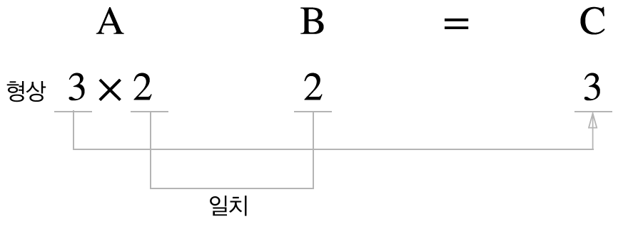
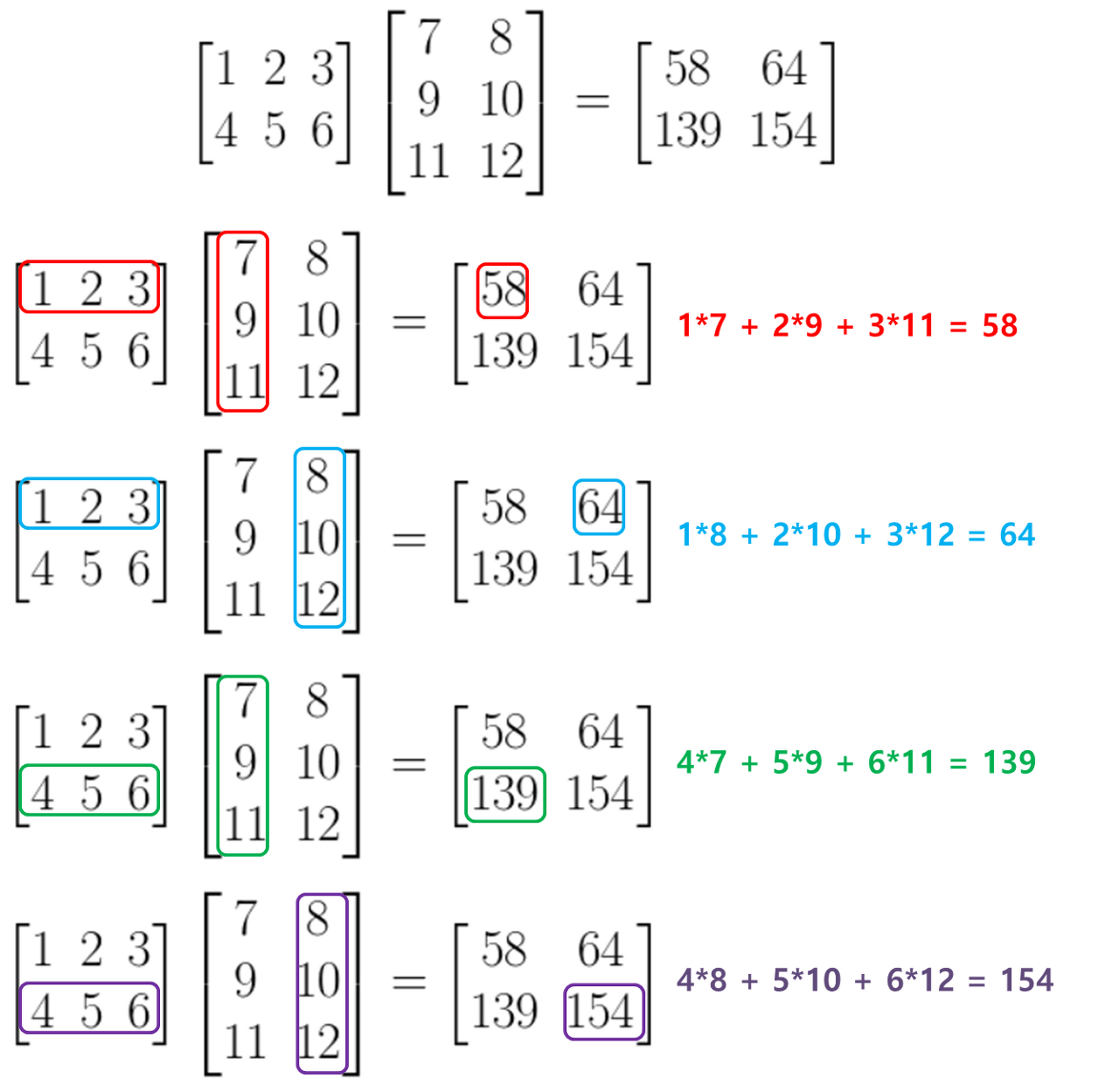
행렬의 내적(행렬 곱)

- 행렬곱 연습


A = np.array([[1,2],[3,4]])
print(A.ndim)
print(A.shape)
print(A.dtype)
B = np.array([[5,6],[7,4]])
print(B.ndim)
print(B.shape)
print(B.dtype)

print(np.dot(A,B))       #A 와 B 내적
#print(np.matmul(A,B))   #(2, 2)(2, 2) --> (2, 2)

A = np.array([[1,2,3], [4,5,6]])
print(A.ndim)
print(A.shape)
print(A.dtype)
B = np.array([[1,2],[3,4],[5,6]])
print(B.ndim)
print(B.shape)
print(B.dtype)

#print(np.dot(A,B))      #A 와 B 내적
print(np.matmul(A,B))    #(2, 3)(3, 2) --> (2, 2)

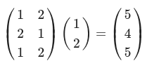
A = np.array([[1,2], [2,1], [1,2]])
print(A.ndim)
print(A.shape)
print(A.dtype)
B = np.array([[1,2,1,2],[2,3,2,3]])
print(B.ndim)
print(B.shape)
print(B.dtype)

#print(np.dot(A,B))      #A 와 B 내적
print(np.matmul(A,B))    #(3, 2)(2, 4) --> (3, 4)
A = np.array([[1,2], [2,1], [1,2]])
print(A.ndim)
print(A.shape)
print(A.dtype)
B = np.array([[1],[2]])
print(B.ndim)
print(B.shape)
print(B.dtype)

#print(np.dot(A,B))      #A 와 B 내적
print(np.matmul(A,B))    #(3, 2)(2, 1) --> (3, 1)
신경망 내적

- X : 입력
- Y : 파라미터

x = np.array([[1,2]])    #(1, 2)
print(x.shape)
W = np.array([[1,3,5],[2,4,6]])     #(2, 3)
print("W:")
print(W)
print(W.shape)
#y = np.dot(x,W) #x 와 W 내적
y = np.matmul(x,W)
print(y)
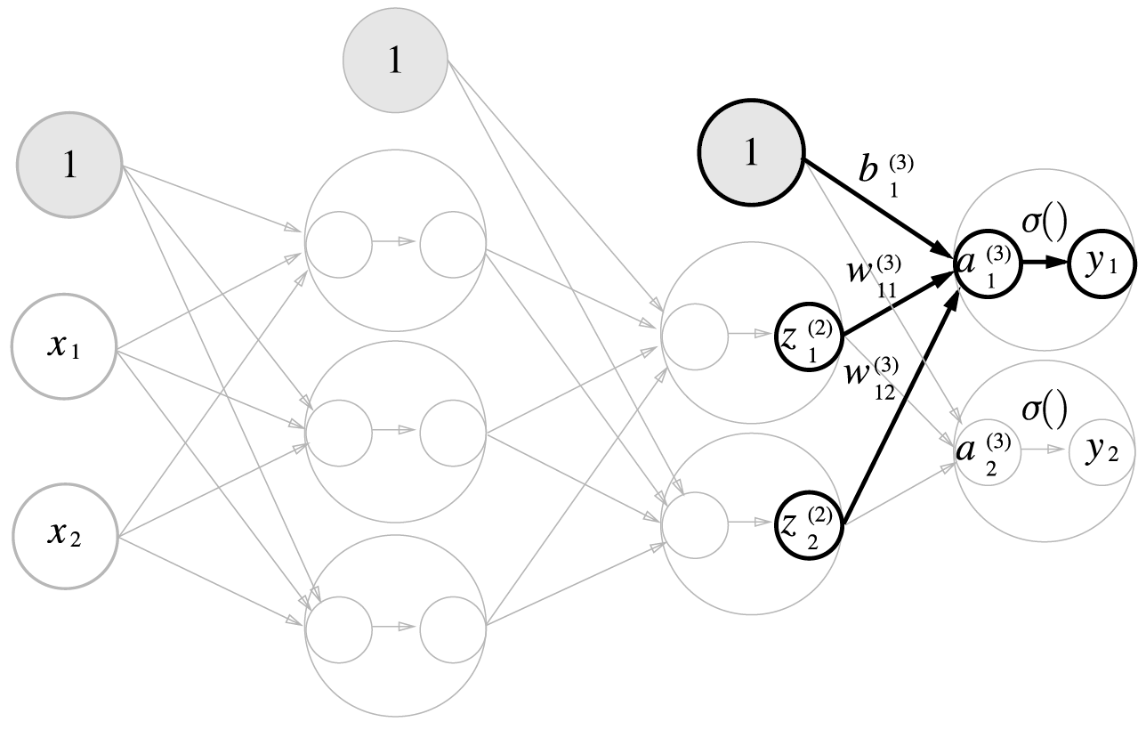
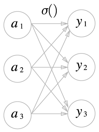
3층 신경망 구현하기
3층 신경망 : 입력층(0층)은 2개, 첫 번째 은닉층(1층)은 3개, 두번째 은닉층(2층)은 2개, 출력층(3층)은 2개의 뉴런으로 구성된다.

표기법 설명

각 층의 신호 전달 구현하기
입력층에서 1층으로 신호 전달


import numpy as np

x = np.array([[1.0,0.5]])
W1 = np.array([[0.1,0.3,0.5],[0.2,0.4,0.6]])
B1 = np.array([[0.1,0.2,0.3]])

print(x.shape)
print(W1.shape)
print(B1.shape)

A1 = np.dot(x,W1) + B1

print(A1)
입력층에서 1층으로의 신호 전달

z1 = sigmoid(A1)

print(z1)
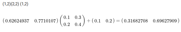
1층에서 2층으로의 신호 전달


W2 = np.array([[0.1, 0.4 ], [0.2, 0.5], [0.3, 0.6]])    # (3, 2)
B2 = np.array([[0.1, 0.2]])
print(z1.shape) # (1, 3)
print(W2.shape) # (3, 2)
print(B2.shape) # (1, 2)
A2 = np.dot(z1, W2) + B2
z2 = sigmoid (A2)
print(A2)
print(z2)
2층에서 출력층으로 신호 전달
def identity_function(x): #항등함수: 입력 그대로 출력으로
  return x

W3 = np.array([[0.1,0.3],[0.2,0.4]])
B3 = np.array([0.1,0.2])

A3 = np.dot(z2,W3) + B3
y = identity_function(A3)
print(y)
구현 정리
def init_network():
    network = {}        #dictionary 형태로 wieght와 bias 저장
    network['W1'] = np.array([[0.1,0.3,0.5],[0.2,0.4,0.6]])
    network['b1'] = np.array([[0.1,0.2,0.3]])
    network['W2'] = np.array([[0.1,0.4],[0.2,0.5],[0.3,0.6]])
    network['b2'] = np.array([[0.1,0.2]])
    network['W3'] = np.array([[0.1,0.3],[0.2,0.4]])
    network['b3'] = np.array([[0.1,0.2]])

    return network

def forward(network,x): #구현된 layer를 따라 데이터 진행
    W1,W2,W3 = network['W1'],network['W2'],network['W3']
    b1,b2,b3 = network['b1'],network['b2'],network['b3']

    a1 = np.dot(x,W1) + b1 #첫번째 layer    (1,2)(2,3) -> (1,3)
    z1 = sigmoid(a1)
    a2 = np.dot(z1,W2) + b2 #두번째 layer      (1,3)(3,2) -> (1,2)
    z2 = sigmoid(a2)
    a3 = np.dot(z2,W3) + b3 #세번째 마지막 layer       (1,2)(2,2) -> (1,2)
    y = identity_function(a3)

    return y

network = init_network()
x = np.array([[1.0,0.5]])
y = forward(network,x)
print(y)
출력층 설계하기
항등 함수와 소프트맥스 함수 구현하기
항등 함수
소프트맥스 함수
- Softmax

- 분자 : 입력 a -> e^a
- 분모 : 입력 a -> e^a -> 전체를 더함
- 분자/분모 ---> 0과 1사이의 값으로 변환, 전체 합은 1

def softmax(a):
    exp_a = np.exp(a)            # 입력에 자연상수(e)를 밑으로 연산 e^a         (분자)
    sum_exp_a = np.sum(exp_a)    # 자연상수(e)를 밑으로 연산 e^a 후 전체를 더함 (분모)
    y = exp_a / sum_exp_a
    return y
소프트맥스 함수 구현 시 주의점
- 지수처리 하면 변수 저장 변위를 쉽게 벗어남(overflow)
- 변수 4byte 또는 8byte
- e^10 -> 20,000 0x4e20
- e^100 -> 10^40개, 자리수 40 이상
- e^1000 -> 무한대처리 inf
- 가장 큰 값으로 빼고 지수 처리하면 overflow를 방지함
- 입력값이 작은 경우 - 정상출력
#a = np.array([1, 2, 3])
#a = np.array([19, 20, 21])
a = np.array([199, 200, 201])
print('input   :', a)
print('exp     :', np.exp(a))
print('exp sum :', np.sum(np.exp(a)))
print('softmax :', np.exp(a)/np.sum(np.exp(a)))- 입력값이 커지면 overflow
a = np.array([1010, 1000, 990])
np.exp(a)/np.sum(np.exp(a))- 최대값을 구한 후 빼기
c=np.max(a)
a-c- overflow 방지
np.exp(a-c)/np.sum(np.exp(a-c))- overflow 방지 softmax 함수
# overflow 방지
def softmax(a):
    c = np.max(a)                 # 배열 a 중 가장 큰 값 선택
    exp_a = np.exp(a-c)
    sum_exp_a = np.sum(exp_a)
    y = exp_a / sum_exp_a
    return y
소프트맥스 함수의 특징
a = np.array([0.3,2.9,4.0])
y = softmax(a)
print(y)
print(np.sum(y))
손글씨 숫자 인식
3.6.1 MNIST 데이터셋
Mnist download
MNIST 이미지 데이터셋의 예
- 0부터 9까지의 숫자 이미지로 구성
- 훈련 이미지 60,000장, 시험 이미지 10,000장
- 훈련 이미지를 사용하여 모델 학습
- 학습한 모델로 시험 이미지들을 얼마나 정확하게 분류하는지 평가

import tensorflow as tf
(x_train,t_train),(x_test,t_test) = tf.keras.datasets.mnist.load_data()

print(x_train.ndim)
print(x_train.shape)
print(x_train.dtype)

x_train = x_train.reshape(60000,-1) #flatten (60000,28,28) - > (60000,784)
x_test = x_test.reshape(10000,-1)
print(x_train.ndim)
print(x_train.shape)
print(x_train.dtype)

print(x_test.ndim)
print(x_test.shape)
print(x_test.dtype)

print(x_train.shape)
print(t_train.shape)
print(x_test.shape)
print(t_test.shape)

from PIL import Image

def img_show(img):
    pil_img = Image.fromarray(np.uint8(img))
    #pll_img.show()
    display(pil_img) # collab에서 실행가능하게 변경

#img = x_train[0]
#label = t_train[0]
#img = x_train[10]
#label = t_train[10]
img = x_train[20]
label = t_train[20]
print(label)
print(img.shape)
img = img.reshape(28,28) #화면에 출력가능한 원래의 이미지 shape으로 변경
print(img.shape)

img_show(img)
- Pickle File
Python Image Library
import pickle

#pickle file 업로드 필요
#with open("/content/drive/MyDrive/Colab Notebooks/deep_learning_start/sample_weight.pkl", 'rb') as f: #저장된 wieght파일을 불러와 출력
#with open("/content/drive/MyDrive/Colab Notebooks/sample_weight.pkl", 'rb') as f: #저장된 wieght파일을 불러와 출력
with open("/content/sample_weight.pkl", 'rb') as f: #저장된 wieght파일을 불러와 출력
    data = pickle.load(f) #binary 형태로 저장되어 있다가 불러오면서 저장당시 class로 복원
#print(data)
print(f"W1: {data['W1']}") #여기서는 dictionary 형태
print(f"b1: {data['b1']}")
신경망의 추론 처리
- Mnist Test
import numpy as np
import pickle
def get_data():
#(x_train, t_train), (x_test, t_test) = load_mnist(normalize=True, flatten=True, one_hot_label=False)
(x_train,t_train),(x_test,t_test) = tf.keras.datasets.mnist.load_data()
x_test = x_test.reshape(10000,-1)
x_test = x_test.astype('float32') / 255. #normalize 데이터를 0과 1사이로
return x_test, t_test
def init_network():
#with open("/content/drive/MyDrive/Colab Notebooks/deep_learning_start/sample_weight.pkl", 'rb') as f: #저장된 wieght파일을 불러와 model에 적용
with open("/content/sample_weight.pkl", 'rb') as f: #저장된 wieght파일을 불러와 model에 적용
network = pickle.load(f)
return network
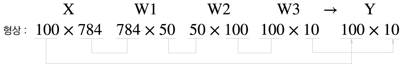
def predict(network, x):
W1, W2, W3 = network['W1'], network['W2'], network['W3'] #위와 같은 3층 layer 구현
b1, b2, b3 = network['b1'], network['b2'], network['b3']
a1 = np.dot(x, W1) + b1 #(100, 784)(784, 50) => (100, 50)
z1 = sigmoid(a1)
a2 = np.dot(z1, W2) + b2 # (100, 50)(50, 100) => (100, 100)
z2 = sigmoid(a2)
a3 = np.dot(z2, W3) + b3 # (100, 100)(100, 10) => (100,10)
y = softmax(a3)
return y
x, t = get_data()
network = init_network()
#print(W1.shape)
#print(W2.shape)
#print(W3.shape)
accuracy_cnt = 0
for i in range(len(x)):
y = predict(network, x[i])
p= np.argmax(y) # 확률이 가장 높은 원소의 인덱스를 얻는다.
if p == t[i]:
accuracy_cnt += 1
print("Accuracy:" + str(float(accuracy_cnt) / len(x)))
print(x[0].shape)

배치처리
Mnist Batch
def get_data():
    #(x_train, t_train), (x_test, t_test) = load_mnist(normalize=True, flatten=True, one_hot_label=False)
    (x_train,t_train),(x_test,t_test) = tf.keras.datasets.mnist.load_data()
    x_test = x_test.reshape(10000,-1)   #
    x_test = x_test.astype('float32') / 255. #normalize 데이터를 0과 1사이로
    return x_test, t_test


def init_network():
    #with open("/content/drive/MyDrive/Colab Notebooks/deep_learning_start/sample_weight.pkl", 'rb') as f:
    with open("/content/sample_weight.pkl", 'rb') as f:
    #with open("/content/drive/MyDrive/data/sample_weight(2).pkl", 'rb') as f:
        network = pickle.load(f)
    return network


def predict(network, x):
    w1, w2, w3 = network['W1'], network['W2'], network['W3']
    b1, b2, b3 = network['b1'], network['b2'], network['b3']

    a1 = np.dot(x, w1) + b1
    z1 = sigmoid(a1)
    a2 = np.dot(z1, w2) + b2
    z2 = sigmoid(a2)
    a3 = np.dot(z2, w3) + b3
    y = softmax(a3)

    return y


x, t = get_data()
network = init_network()

batch_size = 100 # 배치 크기
accuracy_cnt = 0

for i in range(0, len(x), batch_size):
    x_batch = x[i:i+batch_size] # 이미지 1개씩이 아닌 batch size만큼의 이미지를 넘겨줘 한번에 연산
    y_batch = predict(network, x_batch)
    p = np.argmax(y_batch, axis=1)
    accuracy_cnt += np.sum(p == t[i:i+batch_size])

print("Accuracy:" + str(float(accuracy_cnt) / len(x)))
print(x[0:0+batch_size].shape)
행렬

'(두산로보틱스) ROKEY 부트 캠프 > Computer Vision 교육' 카테고리의 다른 글
| ep.42 학습관련기술들 (0) | 2024.09.04 |
|---|---|
| ep.41 신경망학습, 오차역전파법 (0) | 2024.09.03 |
| ep.39 OpenCV5 (0) | 2024.08.30 |
| ep.38 OpenCV4 (0) | 2024.08.29 |
| ep.37 OpenCV3 (0) | 2024.08.28 |


