
printf("ho_tari\n");
ep.33 딥러닝개론7 본문
2024.8.22
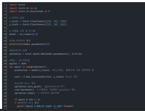
선형회귀

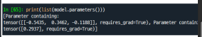
초기선언

경사하강법 사용 학습

자동 미분
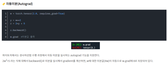
행렬 연산으로 구하기

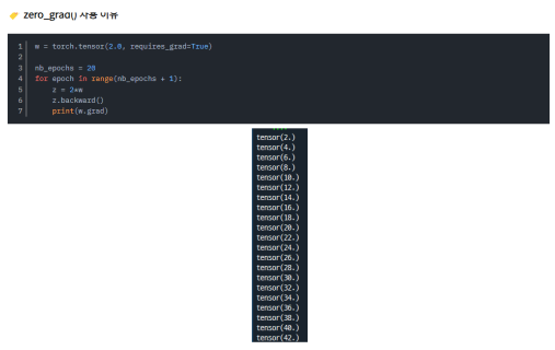
Zero Grad사용 이유
모델 정의 및 학습


Class 사용
파이토치에서는 대부분 클래스를 이용해서 모델을 구현한다.

모델 학습

import torch
import numpy as np
torch.manual_seed(777) # for reproducibility
# Load the data
xy = np.loadtxt('/content/drive/MyDrive/data-04-zoo.csv', delimiter=',', dtype=np.float32)
x_data = xy[:, 0:-1]
y_data = xy[:, [-1]]
print(x_data.shape, y_data.shape)
nb_classes = 7 # 0 ~ 6
# Convert numpy arrays to PyTorch tensors
X = torch.tensor(x_data)
Y = torch.tensor(y_data, dtype=torch.long).view(-1) # Ensure Y is 1D LongTensor for CrossEntropyLoss
# Model definition
model = torch.nn.Linear(16, nb_classes, bias=True)
# Cross entropy loss (which includes softmax)
criterion = torch.nn.CrossEntropyLoss()
optimizer = torch.optim.SGD(model.parameters(), lr=0.1)
for step in range(2001):
optimizer.zero_grad()
hypothesis = model(X)
cost = criterion(hypothesis, Y)
cost.backward()
optimizer.step()
# Prediction
prediction = torch.argmax(hypothesis, 1)
correct_prediction = (prediction == Y)
accuracy = correct_prediction.float().mean()
if step % 100 == 0:
print(f"Step: {step}\tLoss: {cost.item():.3f}\tAcc: {accuracy.item():.2%}")
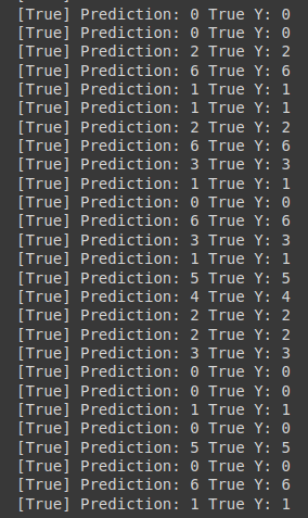
# Let's see if we can predict
pred = torch.argmax(hypothesis, 1)
for p, y in zip(pred, Y):
print(f"[{bool(p.item() == y.item())}] Prediction: {p.item()} True Y: {y.item()}")
# Lab 5 Logistic Regression Classifier
import torch
from torch.autograd import Variable
import numpy as np

torch.manual_seed(777)  # for reproducibility

xy = np.loadtxt('/content/drive/MyDrive/data-03-diabetes.csv', delimiter=',', dtype=np.float32)
x_data = xy[:, 0:-1]
y_data = xy[:, [-1]]

# Make sure the shape and data are OK
print(x_data.shape, y_data.shape)

X = Variable(torch.from_numpy(x_data))
Y = Variable(torch.from_numpy(y_data))

# Hypothesis using sigmoid
linear = torch.nn.Linear(8, 1, bias=True)
sigmoid = torch.nn.Sigmoid()
model = torch.nn.Sequential(linear, sigmoid)

optimizer = torch.optim.SGD(model.parameters(), lr=0.01)

for step in range(10001):
    optimizer.zero_grad()
    hypothesis = model(X)
    # cost/loss function
    cost = -(Y * torch.log(hypothesis) + (1 - Y)
             * torch.log(1 - hypothesis)).mean()
    cost.backward()
    optimizer.step()

    if step % 200 == 0:
        print(step, cost.data.numpy())

# Accuracy computation
predicted = (model(X).data > 0.5).float()
accuracy = (predicted == Y.data).float().mean()
print("\nHypothesis: ", hypothesis.data.numpy(), "\nCorrect (Y): ", predicted.numpy(), "\nAccuracy: ", accuracy)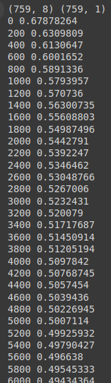


# Lab 5 Logistic Regression Classifier
import torch
from torch.autograd import Variable
import numpy as np

torch.manual_seed(777)

x_data = np.array([[1, 2], [2, 3], [3, 1], [4, 3], [5, 3], [6, 2]], dtype=np.float32)
y_data = np.array([[0], [0], [0], [1], [1], [1]], dtype=np.float32)

X = Variable(torch.from_numpy(x_data))
Y = Variable(torch.from_numpy(y_data))

# Hypothesis using sigmoid: tf.div(1., 1. + tf.exp(tf.matmul(X, W)))
linear = torch.nn.Linear(2, 1, bias=True)
sigmoid = torch.nn.Sigmoid()
model = torch.nn.Sequential(linear, sigmoid)

optimizer = torch.optim.SGD(model.parameters(), lr=0.01)

for step in range(10001):
    optimizer.zero_grad()
    hypothesis = model(X)
    # cost/loss function
    cost = -(Y * torch.log(hypothesis) + (1 - Y)
             * torch.log(1 - hypothesis)).mean()
    cost.backward()
    optimizer.step()

    if step % 200 == 0:
        print(step, cost.data.numpy())


# Accuracy computation
predicted = (model(X).data > 0.5).float()
accuracy = (predicted == Y.data).float().mean()
print("\nHypothesis: ", hypothesis.data.numpy(), "\nCorrect (Y): ", predicted.numpy(), "\nAccuracy: ", accuracy)


# Lab 4 Multi-variable linear regression
import torch
import torch.nn as nn
from torch.autograd import Variable
import numpy as np
torch.manual_seed(777) # for reproducibility
xy = np.loadtxt('/content/drive/MyDrive/data-01-test-score.csv', delimiter=',', dtype=np.float32)
x_data = xy[:, 0:-1]
y_data = xy[:, [-1]]
# Make sure the shape and data are OK
print(x_data.shape, x_data, len(x_data))
print(y_data.shape, y_data)
x_data = Variable(torch.from_numpy(x_data))
y_data = Variable(torch.from_numpy(y_data))
# Our hypothesis XW+b
model = nn.Linear(3, 1, bias=True)
# cost criterion
criterion = nn.MSELoss()
# Minimize
optimizer = torch.optim.SGD(model.parameters(), lr=1e-5)
# Train the model
for step in range(2001):
optimizer.zero_grad()
# Our hypothesis
hypothesis = model(x_data)
cost = criterion(hypothesis, y_data)
cost.backward()
optimizer.step()
if step % 10 == 0:
print(step, "Cost: ", cost.data.numpy(), "\nPrediction:\n", hypothesis.data.numpy())
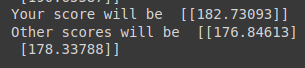
# Ask my score
print("Your score will be ", model(Variable(torch.Tensor([[100, 70, 101]]))).data.numpy())
print("Other scores will be ", model(Variable(torch.Tensor([[60, 70, 110], [90, 100, 80]]))).data.numpy())

# Lab 4 Multi-variable linear regression
import torch
import torch.nn as nn
from torch.autograd import Variable

torch.manual_seed(777)   # for reproducibility

# X and Y data
x_data = [[73., 80., 75.], [93., 88., 93.],
          [89., 91., 90.], [96., 98., 100.], [73., 66., 70.]]
y_data = [[152.], [185.], [180.], [196.], [142.]]

X = Variable(torch.Tensor(x_data))
Y = Variable(torch.Tensor(y_data))

# Our hypothesis XW+b
model = nn.Linear(3, 1, bias=True)

# cost criterion
criterion = nn.MSELoss()
#criterion = nn.CrossEntropyLoss()

# Minimize
optimizer = torch.optim.SGD(model.parameters(), lr=1e-5)

# Train the model
for step in range(2001):
    optimizer.zero_grad()
    # Our hypothesis
    hypothesis = model(X)
    cost = criterion(hypothesis, Y)
    cost.backward()
    optimizer.step()

    if step % 10 == 0:
        print(step, "Cost: ", cost.data.numpy(), "\nPrediction:\n", hypothesis.data.numpy())

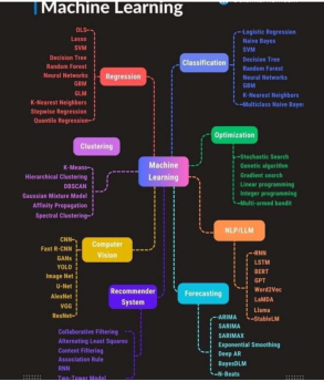
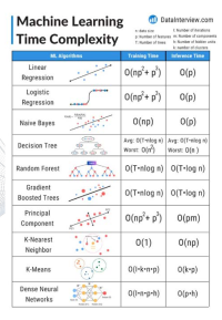
머신러닝
K-Means
• 군집 중심점(centroid)이라는 특정한 임의의 지점을 선택해 해당 중심에 가장 가까운 포인트들을 선택하는 군집화 기법
• 선택된 포인트의 평균지점으로 이동하고 이동된 중심점에서 다시 가까운 포인트를 선택, 다시 중심점을 평균 지점으로 이동하는 프로세스를 반복적으로 수행
• 장점
• 일반적으로 군집화에서 가장 많이 사용되는 알고리즘
• 알고리즘이 쉽고 간결하다
• 단점
• 거리기반 알고리즘으로 속성의 개수가 매우 많을수록 군집화 정확도가 떨어짐 (PCA 차원감소 적용)
• 반복을 수행하는데 반복횟수가 많을 경우 매우 느려짐
• 몇 개의 군집을 선택해야할 지 가이드하기가 어려움

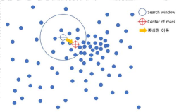
Means Shift
• K 평균과 유사하지만 거리 중심이 아니라 데이터가 모여있는 밀도가 가장 높은 곳으로 군집 중심점을 이동하면서 군집화를 수행함
• 일반 업무 기반의 정형 데이터 세트보다 컴퓨터 비전 영역에서 이미지나 영상 데이터에서 특정 개체를 구분하거나 움직임을 추적하는데 뛰어난 역할을 수행하는 알고리즘이다.
• 이러한 특성 때문에 업무 기반의 데이터 세트보다는 컴퓨터 비전 영역에서 잘 사용된다.
• 장점
•데이터 세트의 형태를 특정 형태로 가정한다든가, 특정 분포도 기반의 모델로 가정하지 않기 때문에 좀 더 유연한 군집화 가능
•이상치의 영향력이 크지 않다
•미리 군집의 개수를 정할 필요가 없다
• 단점
•알고리즘 수행시간이 오래 걸린다
•bandwidth의 크기에 따른 군집화 영향도가 매우 크다
DBSCAN
• DBSCAN(Density Based Spatial Clustering of Applications with Noise)
밀도 기반 군집화의 대표적 예
• 간단하고 직관적인 알고리즘으로 되어 있음에도 데이터의 분포가 기하학적으로 복잡한 데이터 세트에도 효과적인 군집화가 가능
• 특정 공간 내에 데이터 밀도 차이를 기반 알고리즘으로 하고 있어서 복잡한 기하학적 분포도를 가진 데이터 세트에 대해서도 군집화를 잘 수행한다.
• 아래의 복잡한 군집화도 가능!

K-Nearest Neighbor
• 아무튼 K-최근접 이웃 알고리즘의 핵심 내용을 요약해보면 아래와 같이 정리할 수 있다.
• n개의 특성(feature)을 가진 데이터는 n차원의 공간에 점으로 개념화 할 수 있다.
• 유사한 특성을 가진 데이터들끼리는 거리가 가깝다. 그리고 거리 공식을 사용하여 데이터 사이의 거리를 구할 수 있다.
• 분류를 알 수 없는 데이터에 대해 가장 가까운 이웃 k개의 분류를 확인하여 다수결을 할 수 있다.
• 분류기의 효과를 높이기 위해 파라미터를 조정할 수 있다. (K-Nearest Neighbors의 경우 k값을 변경할 수 있다)
• 분류기가 부적절하게 학습되면 overfitting 또는 underfitting이 나타날 수 있다. (K-Nearest Neighbors의 경우 너무 작은 k는 overfitting, 너무 큰 k는 underfitting을 야기한다)

•정규화
• 그래서 K-Means Neighbor 알고리즘을 사용할 때는 모든 특성들을 고르게 반영하기 위해 정규화(Normalization)를 해주곤 한다. 정규화하는 방법에는 여러가지가 있는데, 가장 널리 사용되
는 방법은 두 가지다.
• 최소값을 0, 최대값을 1로 고정한 뒤 모든 값들을 0과 1사이 값으로 변환하는 방법
• 평균과 표준편차를 활용해서 평균으로부터 얼마나 떨어져있는지 z-점수로 변환하는 방법
• 이 외에 다른 방법들도 있고, 각각의 장단점이 있지만 아무튼 보통 위 방법을 적절히 사용
• K개수 선택
• k가 너무 작을 때 : Overfitting
• k가 너무 클 때 : Underfitting
SVM(Support Vector Machine)
• 서포트 벡터 머신(SVM: Support Vector Machine)은 분류와 회귀 과제에 사용할 수 있는 강력한 머신러닝 지도학습 모델
• 서포트 벡터 머신이란
• 서포트 벡터 머신(이하 SVM)은 결정 경계(Decision Boundary), 즉 분류를 위한 기준 선을 정의하는 모델이다. 그래서 분류되지않은 새로운 점이 나타나면 어느 쪽에 속하는지 확인해서 분류 과제를 수행

• 마진
• 마진(Margin)은 결정 경계와 서포트 벡터 사이의 거리를 의미한다.

-최적의 결정 경계는 마진을 최대화한다.
-n개의 속성을 가진 데이터에는 최소 n+1개의 서포트 벡터가 존재한다
-SVM에서는 결정 경계를 정의하는 게 결국 서포트 벡터이기 때문에 데이터 포인트 중에서 서포트 벡터만 잘 골라내면 나머
지 쓸 데 없는 수많은 데이터 포인트들을 무시할 수 있다. 그래서 매우 빠르다.
• Sckit-learn 사용
• Classification: SVC
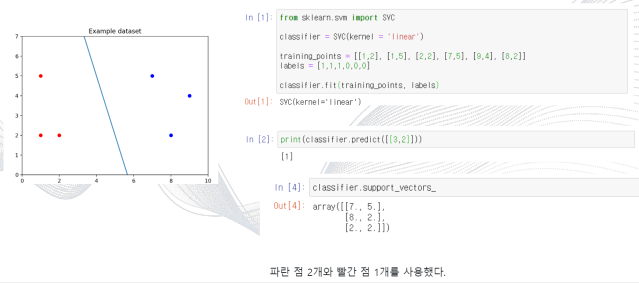
• Regression SVR

SVM 을 회귀에 적용하는 방법은, SVC 와 목표를 반대로 하는 것이다.
•즉, 마진 내부에 데이터가 최대한 많이 들어가도록 학습하는 것이다.
•마진의 폭은 epilson 이라는 하이퍼파라미터를 사용하여 조절한다.
•이상치(Outlier)를 얼마나 허용
• SVM은 데이터 포인트들을 올바르게 분리하면서 마진의 크기를 최대화해야 하는데, 결국 이상치(outlier)를 잘 다루는 게 중요하다.
• 아래 그림을 보자. 선을 살펴보기에 앞서 왼쪽에 혼자 튀어 있는 파란 점과, 오른쪽에 혼자 튀어 있는 빨간 점이 있다는 걸 봐두자. 누가 봐도 아웃라이어다

• 파라미터 C
• 그리고 scikit-learn에서는 SVM 모델이 오류를 어느정도 허용할 것인지 파라미터 C를 통해 지정할 수 있다. (기본값은 1이다.)

'(두산로보틱스) ROKEY 부트 캠프 > Computer Vision 교육' 카테고리의 다른 글
| ep.35 OpenCV1 (0) | 2024.08.26 |
|---|---|
| ep.34 딥러닝개론8 (0) | 2024.08.23 |
| ep.32 딥러닝개론6 (0) | 2024.08.21 |
| ep.31 딥러닝개론5 (0) | 2024.08.20 |
| ep.30 딥러닝개론4 (0) | 2024.08.19 |


