
printf("ho_tari\n");
ep.34 딥러닝개론8 본문
2024.8.23
머신러닝
linearregression.py
import numpy as np
import tensorflow as tf
from tensorflow.keras.models import Sequential
from tensorflow.keras.layers import Dense

# 데이터 생성
np.random.seed(0)
X = np.random.rand(100, 1)  # 100개의 샘플, 1개의 feature
y = 3 * X + 2 + np.random.randn(100, 1) * 0.1  # y = 3x + 2 + 잡음

# 모델 정의
model = Sequential()
model.add(Dense(1, input_dim=1, activation='linear'))

# 모델 컴파일
model.compile(optimizer='sgd', loss='mse')

# 모델 학습
model.fit(X, y, epochs=100, verbose=1)

# 예측
pred = model.predict(X)
logisticregression.py
import numpy as np
import tensorflow as tf
from tensorflow.keras.models import Sequential
from tensorflow.keras.layers import Dense

# 데이터 생성
np.random.seed(0)
X = np.random.randn(100, 1)
y = (X > 0).astype(int)  # 0 또는 1로 변환

# 모델 정의
model = Sequential()
model.add(Dense(1, input_dim=1, activation='sigmoid'))

# 모델 컴파일
model.compile(optimizer='sgd', loss='binary_crossentropy', metrics=['accuracy'])

# 모델 학습
model.fit(X, y, epochs=100, verbose=1)

# 예측
pred = model.predict(X)
force-L.py
import numpy as np
import gym

# 환경 설정 (OpenAI Gym의 FrozenLake 환경)
env = gym.make("FrozenLake-v1", is_slippery=False)

# Q-테이블 초기화
q_table = np.zeros([env.observation_space.n, env.action_space.n])

# 학습 파라미터
alpha = 0.8    # 학습률
gamma = 0.95   # 할인률
epsilon = 0.1  # 탐험(exploration) 확률
episodes = 1000

# Q-learning 알고리즘
for i in range(episodes):
    state = env.reset()
    # 만약 state가 튜플이면 첫 번째 값을 사용
    if isinstance(state, tuple):
        state = state[0]
    done = False

    while not done:
        # 상태 값의 유효성 확인
        if not (0 <= state < q_table.shape[0]):
            print(f"Invalid state: {state}")
            break

        # ε-greedy 정책에 따라 행동 선택
        if np.random.uniform(0, 1) < epsilon:
            action = env.action_space.sample()  # 무작위 행동 선택
        else:
            action = np.argmax(q_table[state])  # Q-값이 가장 큰 행동 선택

        # 환경과 상호작용
        next_state, reward, terminated, truncated, _ = env.step(action)
        # 만약 next_state가 튜플이면 첫 번째 값을 사용
        if isinstance(next_state, tuple):
            next_state = next_state[0]

        # Q-테이블 업데이트
        q_table[state, action] = q_table[state, action] + alpha * (reward + gamma * np.max(q_table[next_state]) - q_table[state, action])

        # 상태 업데이트
        state = next_state
        done = terminated or truncated  # 에피소드 종료 조건

print("학습된 Q-테이블:")
print(q_table)
Supervised-L.py
from sklearn.datasets import load_iris
from sklearn.model_selection import train_test_split
from sklearn.neighbors import KNeighborsClassifier
from sklearn.metrics import accuracy_score

# 데이터 로드
iris = load_iris()
X, y = iris.data, iris.target

# 데이터셋 분리 (학습 데이터와 테스트 데이터)
X_train, X_test, y_train, y_test = train_test_split(X, y, test_size=0.3, random_state=42)

# K-최근접 이웃 분류기 (KNN) 모델 생성 및 학습
model = KNeighborsClassifier(n_neighbors=3)
model.fit(X_train, y_train)

# 예측 및 정확도 계산
y_pred = model.predict(X_test)
print(f'Accuracy: {accuracy_score(y_test, y_pred)}')
unsupervised.py
from sklearn.datasets import load_iris
from sklearn.cluster import KMeans
import matplotlib.pyplot as plt
import pandas as pd

# 데이터 로드
iris = load_iris()
X = iris.data

# K-Means 클러스터링 (k=3)
kmeans = KMeans(n_clusters=3, random_state=42)
y_kmeans = kmeans.fit_predict(X)

# 시각화 (두 개의 차원만 사용)
plt.scatter(X[:, 0], X[:, 1], c=y_kmeans, cmap='viridis')
plt.scatter(kmeans.cluster_centers_[:, 0], kmeans.cluster_centers_[:, 1], s=200, c='red', marker='X')
plt.xlabel(iris.feature_names[0])
plt.ylabel(iris.feature_names[1])
plt.title("K-Means Clustering")
plt.show()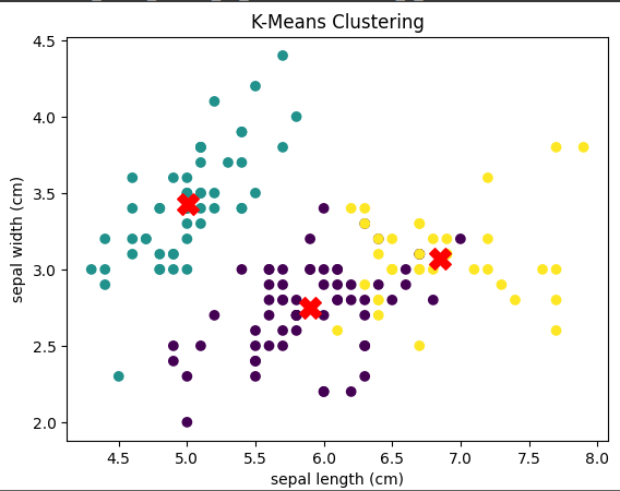
PCA-classify.py
from sklearn.datasets import load_iris
from sklearn.model_selection import train_test_split
from sklearn.decomposition import PCA
from sklearn.neighbors import KNeighborsClassifier
from sklearn.metrics import accuracy_score, classification_report

# 데이터셋 로드
iris = load_iris()
X = iris.data
y = iris.target

# PCA로 차원 축소 (4차원 -> 2차원)
pca = PCA(n_components=2)
X_pca = pca.fit_transform(X)

# 데이터셋 분할 (80% 학습, 20% 테스트)
X_train, X_test, y_train, y_test = train_test_split(X_pca, y, test_size=0.2, random_state=42)

# KNN 분류 모델 정의 (k=3)
knn_classifier = KNeighborsClassifier(n_neighbors=3)

# 모델 학습
knn_classifier.fit(X_train, y_train)

# 예측
y_pred = knn_classifier.predict(X_test)

# 정확도 및 분류 보고서 출력
print("Accuracy:", accuracy_score(y_test, y_pred))
print("\nClassification Report:\n", classification_report(y_test, y_pred))
knn-classifier.py
from sklearn.datasets import load_iris
from sklearn.model_selection import train_test_split
from sklearn.neighbors import KNeighborsClassifier
from sklearn.metrics import accuracy_score, classification_report

# 데이터셋 로드
iris = load_iris()
X = iris.data
y = iris.target

# 데이터셋 분할 (80% 학습, 20% 테스트)
X_train, X_test, y_train, y_test = train_test_split(X, y, test_size=0.2, random_state=42)

# KNN 분류 모델 정의 (k=3)
knn_classifier = KNeighborsClassifier(n_neighbors=3)

# 모델 학습
knn_classifier.fit(X_train, y_train)

# 예측
y_pred = knn_classifier.predict(X_test)

# 정확도 및 분류 보고서 출력
print("Accuracy:", accuracy_score(y_test, y_pred))
print("\nClassification Report:\n", classification_report(y_test, y_pred))
tor-logisticregress.py
import torch
import torch.nn as nn
import torch.optim as optim

# 데이터 생성
torch.manual_seed(0)
X = torch.randn(100, 1)
y = (X > 0).float()  # 0 또는 1로 변환

# 모델 정의
class LogisticRegressionModel(nn.Module):
    def __init__(self):
        super(LogisticRegressionModel, self).__init__()
        self.linear = nn.Linear(1, 1)

    def forward(self, x):
        return torch.sigmoid(self.linear(x))

model = LogisticRegressionModel()

# 손실 함수와 옵티마이저 정의
criterion = nn.BCELoss()
optimizer = optim.SGD(model.parameters(), lr=0.01)

# 모델 학습
for epoch in range(100):
    model.train()

    # 예측값 계산
    y_pred = model(X)

    # 손실 계산
    loss = criterion(y_pred, y)

    # 역전파
    optimizer.zero_grad()
    loss.backward()
    optimizer.step()

    if (epoch + 1) % 10 == 0:
        print(f'Epoch {epoch+1}, Loss: {loss.item()}')

# 예측
pred = model(X).detach().numpy()
knn-diabets.py
from sklearn.datasets import load_diabetes
from sklearn.model_selection import train_test_split
from sklearn.neighbors import KNeighborsRegressor
from sklearn.metrics import mean_squared_error, r2_score

# 데이터셋 로드
diabetes = load_diabetes()
X = diabetes.data
y = diabetes.target

# 데이터셋 분할 (80% 학습, 20% 테스트)
X_train, X_test, y_train, y_test = train_test_split(X, y, test_size=0.2, random_state=42)

# KNN 회귀 모델 정의 (k=5)
knn_regressor = KNeighborsRegressor(n_neighbors=5)

# 모델 학습
knn_regressor.fit(X_train, y_train)

# 예측
y_pred = knn_regressor.predict(X_test)

# MSE 및 R^2 점수 출력
print("Mean Squared Error:", mean_squared_error(y_test, y_pred))
print("R^2 Score:", r2_score(y_test, y_pred))
rmspropanimation.py
import numpy as np
import matplotlib.pyplot as plt
import matplotlib.animation as animation

# 최적화할 함수 (2D)
def func(x, y):
    return x**2 + y**2

# 기울기 계산 (2D)
def gradient(x, y):
    return 2*x, 2*y

# RMSprop 애니메이션
def rmsprop_animation():
    fig, ax = plt.subplots()
    x, y = np.meshgrid(np.linspace(-2, 2, 100), np.linspace(-2, 2, 100))
    z = func(x, y)
    ax.contour(x, y, z, levels=50)

    # 초기 위치
    pos = np.array([1.5, 1.5])
    learning_rate = 0.1
    decay_rate = 0.9
    epsilon = 1e-8

    # 기울기 제곱의 이동 평균
    grad_squared_avg = np.zeros_like(pos)

    point, = ax.plot([], [], 'ro')
    path, = ax.plot([], [], 'r-', alpha=0.5)

    positions = [pos.copy()]

    def update(i):
        nonlocal pos, grad_squared_avg
        grad = np.array(gradient(pos[0], pos[1]))

        # 기울기 제곱의 이동 평균 업데이트
        grad_squared_avg = decay_rate * grad_squared_avg + (1 - decay_rate) * grad**2

        # 학습률 조정
        adjusted_lr = learning_rate / (np.sqrt(grad_squared_avg) + epsilon)

        # 위치 업데이트
        pos -= adjusted_lr * grad
        positions.append(pos.copy())

        # pos 값을 시퀀스로 전달
        point.set_data([pos[0]], [pos[1]])
        path.set_data(*zip(*positions))
        return point, path

    ani = animation.FuncAnimation(fig, update, frames=50, interval=200, blit=True)
    ani.save('/content/rmsprop_animation.gif', writer='pillow')
    plt.close()

    from IPython.display import Image
    return Image('/content/rmsprop_animation.gif')

# 애니메이션 실행
rmsprop_animation()
adamanimation.py
import numpy as np
import matplotlib.pyplot as plt
import matplotlib.animation as animation

# 최적화할 함수 (2D)
def func(x, y):
    return x**2 + y**2

# 기울기 계산 (2D)
def gradient(x, y):
    return 2*x, 2*y

# Adam 애니메이션
def adam_animation():
    fig, ax = plt.subplots()
    x, y = np.meshgrid(np.linspace(-2, 2, 100), np.linspace(-2, 2, 100))
    z = func(x, y)
    ax.contour(x, y, z, levels=50)

    # 초기 위치
    pos = np.array([1.5, 1.5])
    learning_rate = 0.1
    beta1 = 0.9  # 모멘텀을 위한 지수 평균 가중치
    beta2 = 0.999  # 기울기 제곱의 지수 평균 가중치
    epsilon = 1e-8  # 분모 안정화를 위한 작은 값

    m = np.zeros_like(pos)  # 모멘텀(1차 모멘트) 초기화
    v = np.zeros_like(pos)  # 스케일링(2차 모멘트) 초기화
    t = 0  # 타임스텝

    point, = ax.plot([], [], 'ro')
    path, = ax.plot([], [], 'r-', alpha=0.5)

    positions = [pos.copy()]

    def update(i):
        nonlocal pos, m, v, t
        t += 1
        grad = np.array(gradient(pos[0], pos[1]))

        # 모멘텀과 스케일링 업데이트
        m = beta1 * m + (1 - beta1) * grad
        v = beta2 * v + (1 - beta2) * (grad ** 2)

        # 편향 보정
        m_hat = m / (1 - beta1**t)
        v_hat = v / (1 - beta2**t)

        # 위치 업데이트
        pos -= learning_rate * m_hat / (np.sqrt(v_hat) + epsilon)
        positions.append(pos.copy())

        point.set_data([pos[0]], [pos[1]])
        path.set_data(*zip(*positions))
        return point, path

    ani = animation.FuncAnimation(fig, update, frames=50, interval=200, blit=True)
    ani.save('/content/adam_animation.gif', writer='pillow')
    plt.close()

    from IPython.display import Image
    return Image('/content/adam_animation.gif')

# 애니메이션 실행
adam_animation()
adamgradanimation.py
import numpy as np
import matplotlib.pyplot as plt
import matplotlib.animation as animation

# 최적화할 함수 (2D)
def func(x, y):
    return x**2 + y**2

# 기울기 계산 (2D)
def gradient(x, y):
    return 2*x, 2*y

# Adagrad 애니메이션
def adagrad_animation():
    fig, ax = plt.subplots()
    x, y = np.meshgrid(np.linspace(-2, 2, 100), np.linspace(-2, 2, 100))
    z = func(x, y)
    ax.contour(x, y, z, levels=50)

    # 초기 위치
    pos = np.array([1.5, 1.5])
    learning_rate = 1.0
    epsilon = 1e-8

    # 기울기 제곱 합 초기화
    grad_squared_sum = np.zeros_like(pos)

    point, = ax.plot([], [], 'ro')
    path, = ax.plot([], [], 'r-', alpha=0.5)

    positions = [pos.copy()]

    def update(i):
        nonlocal pos, grad_squared_sum
        grad = np.array(gradient(pos[0], pos[1]))

        # 기울기 제곱 합 업데이트
        grad_squared_sum += grad**2

        # 학습률 조정
        adjusted_lr = learning_rate / (np.sqrt(grad_squared_sum) + epsilon)

        # 위치 업데이트
        pos -= adjusted_lr * grad
        positions.append(pos.copy())

        # pos 값을 시퀀스로 전달
        point.set_data([pos[0]], [pos[1]])
        path.set_data(*zip(*positions))
        return point, path

    ani = animation.FuncAnimation(fig, update, frames=50, interval=200, blit=True)
    ani.save('/content/adamgrad_animation.gif', writer='pillow')
    plt.close()

    from IPython.display import Image
    return Image('/content/adamgrad_animation.gif')

# 애니메이션 실행
adagrad_animation()
DR-01408_박성호_딥러닝개론_8차시_수업내용.ipynb
1.17MB
DR-01408_박성호_딥러닝개론_8차시.ipynb
0.05MB
DR-01408_박성호_딥러닝개론_8차시_수업내용.ipynb
1.17MB
DR-01408_박성호_딥러닝개론_8차시.ipynb
0.05MB
'(두산로보틱스) ROKEY 부트 캠프 > Computer Vision 교육' 카테고리의 다른 글
| ep.36 OpenCV2 (0) | 2024.08.27 |
|---|---|
| ep.35 OpenCV1 (0) | 2024.08.26 |
| ep.33 딥러닝개론7 (0) | 2024.08.22 |
| ep.32 딥러닝개론6 (0) | 2024.08.21 |
| ep.31 딥러닝개론5 (0) | 2024.08.20 |
'(두산로보틱스) ROKEY 부트 캠프/Computer Vision 교육' Related Articles
more


